The Heston model is a useful model for simulating stochastic volatility and its effect on the potential paths an asset can take over the life of an option. The Heston model also allows modeling the statistical dependence between the asset returns and the volatility which have been empirically shown to have an inverse relationship. This allows for more effective modeling than the Black-Scholes formula allows due to its restrictive assumption of constant volatility.
Heston Model SDE
The SDE shown below is similar to the standard geometric Brownian motion apart from the fact that the volatility is a stochastic, mean-reverting process. The notation we use here is from Wikipedia.
\(dS_t = \mu S_tdt +\sqrt{v_t}S_tdW_{t}^S\)
\(dv_t = \kappa(\theta - v_t)dt +\xi\sqrt{v_t}dW_{t}^v\)
\(dW_{t}^S\) and \(dW_{t}^v\) are Weiner processes with instantaneous correlation \(\rho\)
\(\mu = \text{drift term}\\ \theta = \text{long run average variance}\\ \kappa= \text{rate of mean reversion}\\ \xi = \text{vol of vol}\\ \)
Generating Correlated Random Normal Variables
To simulate Heston paths we first need to examine how to generate correlated random variables in Python. Let's take a quick example first. Let \(\Sigma\) be the covariance matrix between two random normal variables:
\(\Sigma = \begin{pmatrix}1 & \rho\\\ \rho & 1\end{pmatrix}\)
The means for each random variable are shown below as a vector.
\(\mu = \begin{pmatrix}\mu_1 \\ \mu_2 \end{pmatrix}\)
We can then draw from the following distribution ;
\(W_t\sim\mathcal{N}(\mu, \Sigma)\)
Let's try that in Python and using a rho of -0.70.
import numpy as np
import matplotlib.pyplot as plt

rho = -0.7
Ndraws = 1000
mu = np.array([0,0])
cov = np.array([[1, rho] , [rho , 1]])

W = np.random.multivariate_normal(mu, cov, size=Ndraws)

plt.plot(W.cumsum(axis=0));
plt.title('Correlated Random Variables')
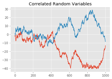
It appears from the plot above that the two processes do in fact move inversely as desired. We can now check statistically whether the desired relationship was created among the variables.
print(np.corrcoef(W.T))

#array([[ 1.        , -0.70388879],
#       [-0.70388879,  1.        ]])
Ok now that we are satisfied that it works we can introduce the concept of stochastic volatility and its relationship to asset returns. In a previous article on the Black-Scholes formula we discussed the problem we assuming that volatility is constant. The Heston model treats the volatility as a random variable which follows an Ornstein–Uhlenbeck process which is nice because it is able to replicate empirically observed properties of volatility.
Properties of Volatility
Mean Reversion
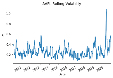
Notice in the plot below for Apple that the volatility never jumps without eventually returning to a certain level, which looks to be approximately 25%.
Recall the notation we introduced at the beginning of the document \( \ \theta \) in this case would be approximately \(0.25^2 = 0.0625\) the rate at which it is pulled towards this long-term variance is \(\kappa\) this behavior makes sense intuitively also since volatility can't go to zero or infinity.
Notice the large spike in volatility in the first quarter of 2020 , it is followed by a return towards some long-term mean that we would need to estimate.
Clustering
Clustering relates to the fact that if volatility is high today it is likely it will be high tomorrow also and vice versa for low volatility periods. In technical terms this means the volatility of a stock exhibits autocorrelation.
Simulating a Heston Process
Essentially what we are doing here is just simulating a standard geometric Brownian motion with non-constant volatility, where the change in S has relationship \(\rho\) with the change in volatility. Here we set the drift term \(\mu\) from above to equal the risk free rate \(r\)
\(S_{t+i} = S_t e^{(r - \frac{v_t}{2})dt + \sqrt{v_i} dW_{t}^S }\)
\(v_{t+1} = v_t + \kappa(\theta-v_t)dt + \xi \sqrt{v_t} dW_t^v\)
So clearly we need to decide on an initial value of \(v_0\) which possibly could be estimated by using a 30 period window. The initial value for \(S_0\) is obviously just the price we observe currently in the market.
Note that in that code we have assured that \(v\) is strictly positive as negative variance values aren't logical. Therefore where you see \(v \ \text{above think} \ |v|\)
def generate_heston_paths(S, T, r, kappa, theta, v_0, rho, xi,
                          steps, Npaths, return_vol=False):
    dt = T/steps
    size = (Npaths, steps)
    prices = np.zeros(size)
    sigs = np.zeros(size)
    S_t = S
    v_t = v_0
    for t in range(steps):
        WT = np.random.multivariate_normal(np.array([0,0]),
                                           cov = np.array([[1,rho],
                                                          [rho,1]]),
                                           size=Npaths) * np.sqrt(dt)

        S_t = S_t*(np.exp( (r- 0.5*v_t)*dt+ np.sqrt(v_t) *WT[:,0] ) )
        v_t = np.abs(v_t + kappa*(theta-v_t)*dt + xi*np.sqrt(v_t)*WT[:,1])
        prices[:, t] = S_t
        sigs[:, t] = v_t

    if return_vol:
        return prices, sigs

    return prices
We can now generate paths for a Heston process, the paths below were generated with an annual volatility of 20%. The Python snippet to plot paths for a Heston process is given at the end of the document to avoid clutter, see 'plotting paths of a Heston process' for the parameters used for this demonstration.
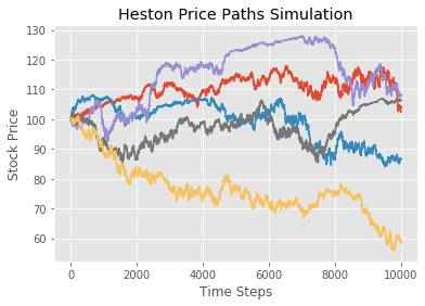
We used a \(\kappa\) of 3 here, chosen for convenience. In practice these parameters would mostly likely be estimated from market prices. Perhaps we will create a separate article on how that is done.
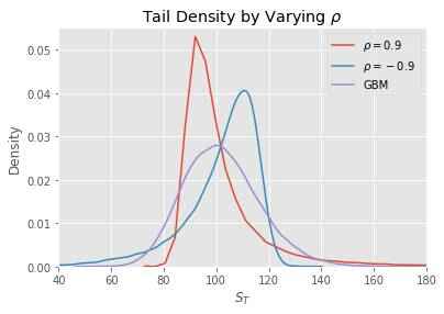
Let's take a look at different distributions of \(S_T\) when varying the correlation measure \(\rho\) between the Weiner processes.
kappa =4
theta = 0.02
v_0 =  0.02
xi = 0.9
r = 0.02
S = 100
paths =50000
steps = 2000
T = 1

prices_pos = generate_heston_paths(S, T, r, kappa, theta,
                                    v_0, rho=0.9, xi=xi, steps=steps, Npaths=paths,
                                    return_vol=False)[:,-1]
prices_neg  = generate_heston_paths(S, T, r, kappa, theta,
                                    v_0, rho=-0.9, xi=xi, steps=steps, Npaths=paths,
                                    return_vol=False)[:,-1]
gbm_bench = S*np.exp( np.random.normal((r - v_0/2)*T ,
                                np.sqrt(theta)*np.sqrt(T), size=paths))

import seaborn as sns

fig, ax = plt.subplots()

ax = sns.kdeplot(data=prices_pos, label=r"$\rho = 0.9$", ax=ax)
ax = sns.kdeplot(data=prices_neg, label=r"$\rho= -0.9$ ", ax=ax)
ax = sns.kdeplot(data=gbm_bench, label="GBM", ax=ax)

ax.set_title(r'Tail Density by Varying $\rho$')
plt.axis([40, 180, 0, 0.055])
plt.xlabel('$S_T$')
plt.ylabel('Density')
Pricing Options with Heston Model
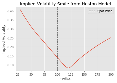
Let's take the terminal prices we got from the simulation above when \(\rho = 0.9\) and price options for a range of strikes. We will price a chain of puts between 30 - 200$. And investigate whether we get a volatility smile. To run the script below you will need the BS_CALL, BS_PUT and implied_vol function from this article on the subject.
strikes =np.arange(30, 200,1)

puts = []

for K in strikes:
    P = np.mean(np.maximum(K-prices_neg,0))*np.exp(-r*T)
    puts.append(P)


ivs = [implied_vol(P, S, K, T, r, type_ = 'put' ) for P, K in zip(puts,strikes)]

plt.plot(strikes, ivs)
plt.ylabel('Implied Volatility')
plt.xlabel('Strike')
plt.axvline(S, color='black',linestyle='--',
            label='Spot Price')
plt.title('Implied Volatility Smile from Heston Model')
plt.legend()
It appears we do in fact get a volatility smile as expected, albeit a rather weird looking one. This is probably due to the unrealistically high correlation we have used in this example. We will leave it to the reader to play around with these parameters and inspect the resulting smiles.
As mentioned previously Heston derived a closed form solution, which is necessary in order to calibrate the model to market prices as we have shown for the Merton jump diffusion model.
So to summarize, clearly the Heston model is an improvement on the Black-Scholes model, due to the ability to model volatility as a mean-reverting random variable.
It may be interesting to try to incorporate jumps to both the stock return and the volatility, perhaps trying to model stochastic correlation may be an interesting topic also. All of which we will endeavor to cover in future articles.
Plotting Paths of Heston Process
kappa =3
theta = 0.04
v_0 = 0.04
xi = 0.6
r = 0.05
S = 100
paths =3
steps = 10000
T = 1
rho = -0.8
prices,sigs = generate_heston_paths(S, T, r, kappa, theta,
v_0, rho, xi, steps, paths,
return_vol=True)
plt.figure(figsize=(7,6))
plt.plot(prices.T)
plt.title('Heston Price Paths Simulation')
plt.xlabel('Time Steps')
plt.ylabel('Stock Price')
plt.show()
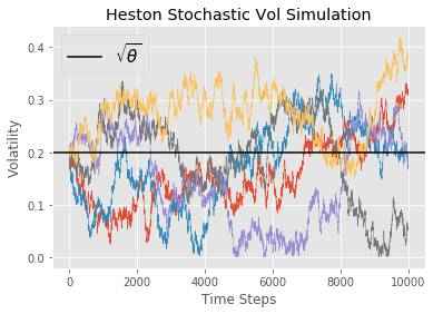
plt.figure(figsize=(7,6))
plt.plot(np.sqrt(sigs).T)
plt.axhline(np.sqrt(theta), color='black', label=r'$\sqrt{\theta}$')
plt.title('Heston Stochastic Vol Simulation')
plt.xlabel('Time Steps')
plt.ylabel('Volatility')
plt.legend(fontsize=15)
plt.show()