The Black-Scholes equations revolutionized option pricing when the paper was published by Mryon Scholes and Fischer Black in 1973. The arguments they use in their paper also follow no arbitrage arguments which were discussed here. We present the formulae here without derivation, which will be provided in a separate article. We can also simulate the Black-Scholes model as shown here.
Contents
- Assumptions of Black Scholes
- Non-dividend paying stock formula and Python implementation
- Parameter effects on option values
- Dividend paying stock implementation
- OOP implementation.
Black-Scholes Assumptions
There are a number of important assumptions to consider when viewing the formulae below.
1) Interest rate is known and constant through time.
2) The stock follows a random walk in continuous time, the variance of the stock price paths follow a log-normal distribution.
3) Volatility is constant
4) Stock pays no dividends (can be modified to include them however)
5) The option can only be exercised at expiration i.e. it is a European type option.
6) No transaction costs i.e. fees on shorting selling etc.
7) Fractional trading is possible i.e. we can buy/sell 0.x of any given stock.
Black Scholes Formula for Non Dividend Paying Stock
The formulae for both the put and the call is given below.
\(Call = S_{0}N(d_1) - N(d_2)Ke^{-rT}\)
\(Put=N(-d_2)Ke^{-rT} - N(-d_1)S_0\)
\(\\d_1 = \frac{ln(\frac{S}{K}) + (r + \frac{\sigma^2}{2})T}{\sigma\sqrt{T}} \\ \\d_2 =d_1 - \sigma\sqrt{T}\)
S : current asset price
K: strike price of the option
r: risk free rate
T : time until option expiration
σ: annualized volatility of the asset's returns
N(x): is the cumulative distribution function for a standard normal distribution shown below.
\(N(x) =\displaystyle \int_{-\infty}^{x} \frac{e^{-x^{2}/2}} {\sqrt{2\pi}}\)
import numpy as np
from scipy.stats import norm

N = norm.cdf

def BS_CALL(S, K, T, r, sigma):
    d1 = (np.log(S/K) + (r + sigma**2/2)*T) / (sigma*np.sqrt(T))
    d2 = d1 - sigma * np.sqrt(T)
    return S * N(d1) - K * np.exp(-r*T)* N(d2)

def BS_PUT(S, K, T, r, sigma):
    d1 = (np.log(S/K) + (r + sigma**2/2)*T) / (sigma*np.sqrt(T))
    d2 = d1 - sigma* np.sqrt(T)
    return K*np.exp(-r*T)*N(-d2) - S*N(-d1)
In this section we will examine the effects of changing the input parameters to the value of calls and puts.
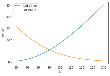
S Effect on Option Value
Here we will hold constant all the variables except the current stock price S and examine how the value of calls and puts change.
K = 100
r = 0.1
T = 1
sigma = 0.3

S = np.arange(60,140,0.1)

calls = [BS_CALL(s, K, T, r, sigma) for s in S]
puts = [BS_PUT(s, K, T, r, sigma) for s in S]
plt.plot(STs, calls, label='Call Value')
plt.plot(STs, puts, label='Put Value')
plt.xlabel('$S_0$')
plt.ylabel(' Value')
plt.legend()
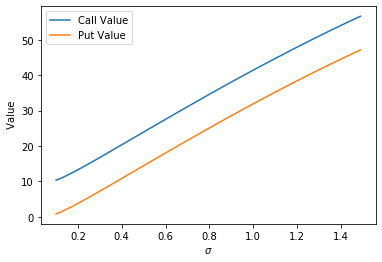
\(\sigma\) Effect on Black-Scholes Value
As we would expect, when we hold the other variables constant, and increase the volatility parameter both calls and puts increase in value, in what appears to be a linear fashion as shown below.
To understand why the calls value seems to be strictly greater than the put with respect to volatility, change the interest rate \(r\) to 0 and notice that the curve coincide exactly. Rather than making plots for the effect on interest rates, we can deduce from this that an increase in interest rates increases the value of calls and decreases the value of puts.
K = 100
r = 0.1
T = 1
Sigmas = np.arange(0.1, 1.5, 0.01)
S = 100

calls = [BS_CALL(S, K, T, r, sig) for sig in Sigmas]
puts = [BS_PUT(S, K, T, r, sig) for sig in Sigmas]
plt.plot(Sigmas, calls, label='Call Value')
plt.plot(Sigmas, puts, label='Put Value')
plt.xlabel('$\sigma$')
plt.ylabel(' Value')
plt.legend()
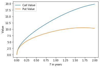
Effect of Time on Black-Scholes Price
As we increase time we increase the uncertainty regarding the future price. Since uncertainty is to the options holder benefit, the price of the option increases with time. Again try setting the interest rate to zero to observe that the difference between puts and calls is eliminated.
K = 100
r = 0.05
T = np.arange(0, 2, 0.01)
sigma = 0.3
S = 100

calls = [BS_CALL(S, K, t, r, sigma) for t in T]
puts = [BS_PUT(S, K, t, r, sigma) for t in T]
plt.plot(T, calls, label='Call Value')
plt.plot(T, puts, label='Put Value')
plt.xlabel('$T$ in years')
plt.ylabel(' Value')
plt.legend()
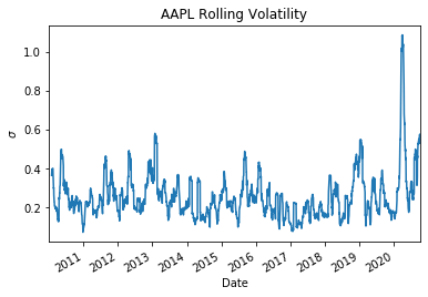
Main Problem with Black Scholes
The script below calculates the rolling standard deviation for APPLE over approximately 10 years. Notice that the volatility is in no way stable, if we take the standard deviation over the entire sample it is approximately 0.28 , however, notice that in early-mid 2020 during there is a large spike. As mentioned, the Black-Scholes model assumes this parameter is constant.
import pandas_datareader.data as web
import pandas as pd
import datetime as dt
import numpy as np
import matplotlib.pyplot as plt

start = dt.datetime(2010,1,1)
end =dt.datetime(2020,10,1)
symbol = 'AAPL' ###using Apple as an example
source = 'yahoo'
data = web.DataReader(symbol, source, start, end)
data['change'] = data['Adj Close'].pct_change()
data['rolling_sigma'] = data['change'].rolling(20).std() * np.sqrt(255)


data.rolling_sigma.plot()
plt.ylabel('$\sigma$')
plt.title('AAPL Rolling Volatility')
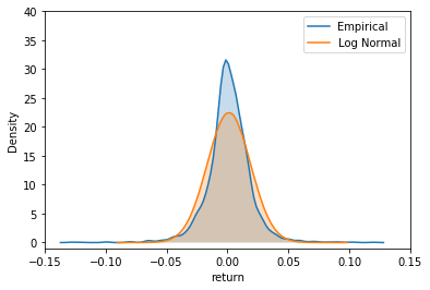
Another key problem is that the model underestimates the tail density. The KDE plot below shows the empirical verus a normal distribution for Apple stock. This means that Black-Scholes will underestimate the value of out-of-the-money options. Both of these problems will be addressed in future articles.
std = data.change.std()
WT = np.random.normal(data.change.mean() ,std, size=Ndraws)
plt.hist(np.exp(WT)-1,bins=300,color='red',alpha=0.4);
plt.hist(data.change,bins=200,color='black', alpha=0.4);
plt.xlim([-0.03,0.03])

import seaborn as sns

fig, ax = plt.subplots()
ax = sns.kdeplot(data=data['change'].dropna(), label='Empirical', ax=ax,shade=True)
ax = sns.kdeplot(data=WT, label='Log Normal', ax=ax,shade=True)
plt.xlim([-0.15,0.15])
plt.ylim([-1,40])
plt.xlabel('return')
plt.ylabel('Density')
Black-Scholes for Dividend Paying Stock
We can easily modify the non-dividend formula described above to include a dividend. Note that the dividend denoted as \(q\) below is a continuously compounded dividend. This means that the actual dividend date is irrelevant to the pricing formula. Clearly this isn't ideal and could result in large errors for stocks which pays large dividends.
\(Call = S_{0}e^{-qT}N(d_1) - N(d_2)Ke^{-rT}\)
\(Put=N(-d_2)Ke^{-rT} - N(-d_1)S_0e^{-qT}\)
\(\\d_1 = \frac{ln(\frac{S}{K}) + (r -q+ \frac{\sigma^2}{2})T}{\sigma\sqrt{T}} \\ \\d_2 =d_1 - \sigma\sqrt{T}\)
def BS_CALLDIV(S, K, T, r, q, sigma):
    d1 = (np.log(S/K) + (r - q + sigma**2/2)*T) / (sigma*np.sqrt(T))
    d2 = d1 - sigma* np.sqrt(T)
    return S*np.exp(-q*T) * N(d1) - K * np.exp(-r*T)* N(d2)

def BS_PUTDIV(S, K, T, r, q, sigma):
    d1 = (np.log(S/K) + (r - q + sigma**2/2)*T) / (sigma*np.sqrt(T))
    d2 = d1 - sigma* np.sqrt(T)
    return K*np.exp(-r*T)*N(-d2) - S*np.exp(-q*T)*N(-d1)
OOP Implementation
Notice that there is a lot of repetitive code in the functions above, we can combine everything into an object orientated program as shown below. To price both a call and put, insert 'B' for both into the price method.
from scipy.stats import norm

class BsOption:
    def __init__(self, S, K, T, r, sigma, q=0):
        self.S = S
        self.K = K
        self.T = T
        self.r = r
        self.sigma = sigma
        self.q = q


    @staticmethod
    def N(x):
        return norm.cdf(x)

    @property
    def params(self):
        return {'S': self.S,
                'K': self.K,
                'T': self.T,
                'r':self.r,
                'q':self.q,
                'sigma':self.sigma}

    def d1(self):
        return (np.log(self.S/self.K) + (self.r -self.q + self.sigma**2/2)*self.T) \
                                / (self.sigma*np.sqrt(self.T))

    def d2(self):
        return self.d1() - self.sigma*np.sqrt(self.T)

    def _call_value(self):
        return self.S*np.exp(-self.q*self.T)*self.N(self.d1()) - \
                    self.K*np.exp(-self.r*self.T) * self.N(self.d2())

    def _put_value(self):
        return self.K*np.exp(-self.r*self.T) * self.N(-self.d2()) -\
                self.S*np.exp(-self.q*self.T)*self.N(-self.d1())

    def price(self, type_ = 'C'):
        if type_ == 'C':
            return self._call_value()
        if type_ == 'P':
            return self._put_value()
        if type_ == 'B':
            return  {'call': self._call_value(), 'put': self._put_value()}
        else:
            raise ValueError('Unrecognized type')


if __name__ == '__main__':
    K = 100
    r = 0.1
    T = 1
    sigma = 0.3
    S = 100
    print(BsOption(S, K, T, r, sigma).price('B'))


#Out:
#{'call': 16.73413358238666, 'put': 7.217875385982609}