In this article we will cover some important topics which are necessary for understanding the most common option pricing models. We will cover the factors determining option prices and also give a brief explanation of the important put-call parity relationship. We will also give an example of pricing puts using put-call parity from real options pricing data.
The concepts covered here will act as an introduction to understanding the parameters that are inputs to famous pricing formulae e.g. Black Scholes & Lattice Methods.
Factors Affecting Option Prices
Moneyness
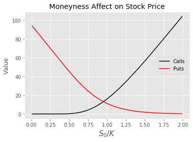
Moneyness can be viewed as the current price of the stock \(S_0\) in relation to the strike price \(K\). Clearly this will affect calls and puts differently.
\(\text{Moneyness} = \frac{S_0}{K}\)
A call option has a positive relationship with moneyness, since higher stock values in relation to the strike indicate the option has more value. The opposite is true for a put option, since the holder of a put option benefits from a decrease in the price of a stock, the higher the strike price in relation to the stock price the higher the value of the option holder's position.
Volatility
Volatility is a major factor in the price of an option. When thinking of volatility it is useful to think of it as the range of potential future stock prices. Since the holder of an option is interested in extreme values due to the fact that we are not obligated to buy the stock at expiration, both calls and puts will benefit from an increase in volatility.
Consider the following short analogous example to understand this concept.
Volatility is calculated on the returns from a stock. Usually the period log returns \(r_i\) are considered.
\(r_i = log(S_t) - log(S_{t-1})\)
We can then calculate the standard deviation \(\sigma\) of returns as shown below where \(\bar{r}\) is the sample mean of the log returns.
\(\sigma =\sqrt{\frac{1}{N-1} \sum r_i - \bar{r} }\)
Another important point regarding volatility is that we often have to annualize it for the purposes of some pricing models. If we have daily closing prices and used the formulae above we would need to annualize it by multiplying by \(\sqrt{255}\) we use 255 as there are approximately 255 trading days in a year. If we were dealing with month-to-month returns we would multiply by \(\sqrt{12}\). The general formula for annualizing volatility is \(\sigma \sqrt{T}\). If you are unsure about why we multiply by the square root of time, this is due to the fact that variance is additive, so consider multiplying the variance by a scalar and then taking the square root.
A loose analogy to the volatility of a stock is the break horse power (BHP) of cars. Say for example we are betting how far a car can travel within a set time. Clearly a car with a higher break horse power has the potential to travel further. Say we have two cars , Car A has a BHP of 500 and Car B has a BHP of 300, now consider drawing a circle around the starting point of each of the cars representing the potential finishing points after x units of time, the circle for Car A should be larger since it has more potential energy. In this example we are assuming that a car moves as quickly in reverse as it does moving in a straight line.
This is a useful analogy to volatility of a stock, think of volatility as the break horse power of a car. Now consider a call option, when purchasing a call you want the stock to move as far as possible over the strike. Stocks with higher volatility will be more profitable.
Looking at the plot below, consider a stock is currently priced at $100 , the brown distribution represents a 30% volatility and the green a 50%, clearly the green distribution offers more extreme and frequent positive / negative values, this would mean we make more money on average when compared to the brown curve.
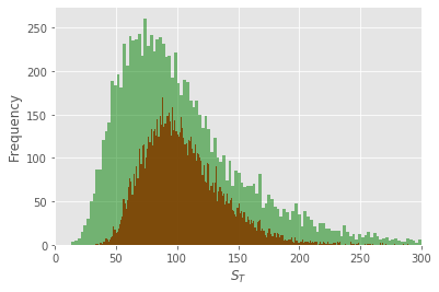
From this we can conclude that volatility has a positive relationship with both calls and puts.
Time to Expiration
Time to expiration usually denoted \(T\) in pricing formulae has a positive relationship with both call and put options. This makes sense intuitively also, since the further away something is the less certain we are about it. It may be useful to return to the section above about annualizing volatility, notice that the uncertainty increase by \(\sqrt{T}\) so therefore longer periods will be inherently more uncertain.
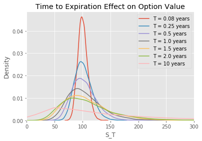
Therefore we can conclude that time has a positive relationship with both calls and puts.
Interest Rates and Dividends
Interest rates have a positive relationship with stock prices generally. This is due to the fact that, if an investor could get say 5% from investing in a savings account or 5% investing in a stock, he would much prefer to invest in the savings account since there is much less uncertainty involved with this investment. So therefore we can conclude that the return from a stock must be at least as high as the return from a savings account.
So an increase in interest rates means we should expect the return on a stock to increase and therefore interest rates and call options have a positive relationship, whereas interest rates and put options move in opposite directions.
Which interest rate should be used to measure this? Well commonly a government bond is used, this is known as the risk-free rate and is usually denoted \(r\) or \(r_f\).
For dividends, let's first consider what happens when a company pays a dividend. Let's say a company announces a $2 dividend to be paid in 1 month's time, Let's say prior to the dividend being paid, the stock is at $100, immediately after payment we would expect the stock to trade for $98 , since $2 of value has been returned to shareholders.
So clearly anything that reduces the stock price increases the value of puts and decreases the value of calls.
Put Call Parity
In this section we will cover an important relationship between calls and puts. In order for markets to be free from arbitrage the following relation between a put \(P\) and a call \(C\) must hold. Note that the put and call should have the same strike \(K\) and time to expiration \(T\).
\(C + Ke^{-rT} = P + S_0\)
If this equality doesn't hold, then a trader could short one side of the equation and buy the other getting a risk free profit, therefore it is assumed that no arbitrage exists in markets. This equality can be useful in a number of ways. Say for instance we are making a pricing model that is computationally intensive, having this equality means we would only need to calculate the price of a call/put and we get the other one by manipulating the equality.
Another interesting application is that we can back out the interest rate implied by the option prices as follows:
\(r = -\frac {ln \left[ \frac{S_0 + P - C}{K} \right]}{T}\)
So let's try that on some market data and see what we get. Usually we would need the dividend rate also in order to get an accurate reading, however, for simplicity we will select a stock that doesn't pay dividends to illustrate the point. Tesla is a good choice for this exercise, the script below downloads all the options available on Yahoo Finance for Tesla. We will also calculate the mid price of the option for each strike/expiry as follows:
\(\text{midpoint} = \frac{Bid + Ask}{2}\)
import pandas as pd
import pandas_datareader.data as web
import numpy as np
import matplotlib.pyplot as plt
plt.style.use('ggplot')

TSLA = web.YahooOptions('TSLA')

alloptions = TSLA.get_all_data()
alloptions.reset_index(inplace=True)

exp1 = alloptions[alloptions.Expiry == TSLA.expiry_dates[1]]

calls = exp1[exp1.Type=='call']
calls['C'] = (calls.Bid+calls.Ask)/2
puts = exp1[exp1.Type=='put']
puts['P'] = (puts.Bid+puts.Ask)/2

df = pd.merge(calls, puts, how='inner', on ='Strike')

df

#    Strike  ...        P
#0    350.0  ...    2.880
#1    360.0  ...    3.275
#2    380.0  ...    4.075
#3    390.0  ...    4.575
#4    400.0  ...    5.150
#..     ...  ...      ...
#65   700.0  ...  125.175
#66   750.0  ...  164.950
#67   800.0  ...  207.750
#68   850.0  ...  252.900
#69   900.0  ...  299.450
#
#[70 rows x 39 columns]
Although this is obviously subject to change depending on when the script is run, there are currently 70 puts and calls with the same Strike for this expiry. We can now try to calculate the price of a put using put-call parity.
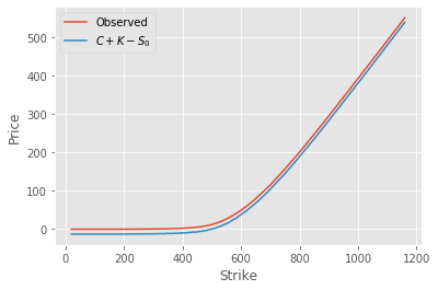
\(P = C + K - S_0\)
df['S'] = df.Underlying_Price_x
df['Parity_P'] = df.C + df.Strike - df.S

%matplotlib inline
plt.plot(df.Strike, df.P, label='Observed')
plt.plot(df.Strike,df.Parity_P, label=r'$C+ K -S_0$')
plt.xlabel('Strike')
plt.ylabel('Price')
plt.legend()
And we can also try to recover the interest rate used.
df['Time'] = (df.Expiry_x - dt.datetime.now()).dt.days / 255
df['r'] = -np.log( (df.S+df.P-df.C)/ df.Strike) / df.Time

plt.figure(figsize=(8,4))
plt.plot(df.Strike, df.r, label=r' $-\frac {ln \left[ \frac{S_0 + P - C}{K} \right]}{T}$')
plt.xlabel('Strike')
plt.ylabel('Interest Rate')
plt.vlines(df.S, df.r.min(), df.r.max(), linestyle='--', label=r'$S_0$')
plt.legend(fontsize=20)
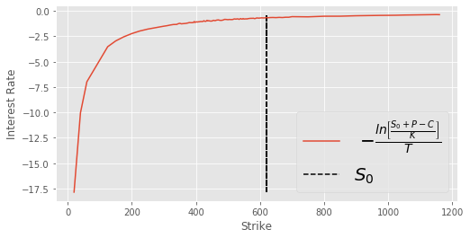
Clearly using real market prices is much messier than a theoretical framework. Perhaps we can attribute the difference in interest rates above due to the higher bid/ask spread observed for deep out of the money options.
Notice below if we include the interest rate parameter there is no difference between the put-call parity implied prices and the market observable prices.
df['Parity_P2'] = df.C+df.Strike*np.exp(-df.r*df.Time) - df.S
plt.plot(df.Strike, df.P, label='Observed')
plt.plot(df.Strike,df.Parity_P2, label=r'$C+Ke^{-rT} - S_0$')
plt.legend()
In the next article we will discuss ways to price options using some well known models.