The Merton Jump diffusion model is a result of Robert C. Merton's 1979 paper Option Pricing When Underlying Stock Returns Are Discountious. The main idea regarding this paper was to extend the Black-Scholes model to incorporate more realistic assumptions and that deal with the fact that empirical studies of market returns, do not follow a constant variance log-normal distribution.
The Merton jump diffusion model is also interesting due to the fact that it is able to produce the volatility smile which is observed in all options markets. Jumps are often one of the explanations for the presence of this smile.
In this article we will investigate the following:
1) How to simulate a jump diffusion process
2) Python implementation of Merton's formula to see if we can produce a volatility smile from artificial data.
3) Model calibration to market prices to find optimal parameters using least squares.
In this article we won't go into too much detail regarding proofs etc, we highly recommend reading Merton's original paper available in pdf here. The notation we follow in this article was created referencing to this Wolfram post on the topic, as the notation is more accessible.
Notation Used Throughout this Article
\(S = \text{Current Stock Price} \\ K = \text{Strike} \\ T= \text{Time to maturity in years} \\ \sigma = \text{Annual Volatility} \\ m = \text{Mean of Jump Size} \\ v = \text{Standard Deviation of Jump Size} \\ \lambda = \text{Number of jumps per year (intensity)}\\ \text{dW(t)} = \text{Weiner Process}\\ N(t) = \text{Compound Poisson Process} \\ V_{BS} = \text{Value of option using Black-Scholes Formula}\\ V_{MJD} = \text{Value of option using Merton Jump Diffusion Model} \)
Jump Diffusion SDE
Merton distinguishes between the following two types of change in stock prices.
Normal vibrations in price
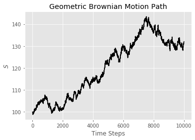
Examples of which include imbalance between supply and demand etc. These changes are well suited to being modeled by geometric Brownian motion. The following article on simulating options prices may be useful to see a Python example and more details regarding this type of process. The integral below is for simulating geometric Brownian motion paths.
\(ln(S_{T}) = ln(S) + \displaystyle \int_{0}^t(r - \frac{\sigma^2}{2})dt + \displaystyle \int_{0}^t \sigma dW(t) \)
The image below shows a single random path of a stock that follows the process above.
Abnormal vibrations in price
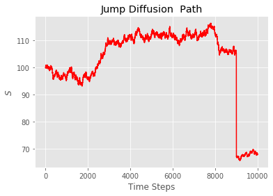
These are the changes that Merton describes as discontinuous. These are changes that would be effectively impossible when using geometric Brownian motions paths as shown below. But of course such large changes do occur in the market, not too infrequently. Examples of these discontinuities could be natural disasters, corporate scandals, earnings season or mergers & acquisitions etc. Notice that there is just one term added to the SDE below, adding an extra source of randomness to account for the aforementioned discontinuities.
\(ln(S_{T}) = ln(S) + \displaystyle \int_{0}^t(r - \frac{\sigma^2}{2})dt + \displaystyle \int_{0}^t \sigma dW(t) + \displaystyle \sum_{j=1}^{N_t} (Q_j-1)\)
Where \(N(t)\) is a Poison Process with probability of \(k\) jumps occurring over the life of the option equal to \(\mathbb{P}(N(t) =k) = \frac{(\lambda t)^k e^{-\lambda t}}{k!}\)and \(Q_j\) is a log-normally distributed random variable.
Below is an example of a jump diffusion path, clearly the long vertical line at approximately step 9000 is the discontinuous behavior we have discussed.
Python Snippet to Simulate Jump Diffusion
Note that in the code below this part \(\displaystyle \int_{0}^t(r - \frac{\sigma^2}{2})dt\) of the integral from the section at the beginning of this document as been adjusted to \(\displaystyle \int_{0}^t(r - \frac{\sigma^2 }{2} - \lambda(m+\frac{v^2}{2}))dt\) so we can write the jump component as a normal random variable and the resulting payoffs will be risk neutral.
Basically this was done as it makes the coding easier and make it easy to benchmark against Merton's formula which will be discussed in the next section.
import matplotlib.pyplot as plt
plt.style.use('ggplot')
import numpy as np
def merton_jump_paths(S, T, r, sigma, lam, m, v, steps, Npaths):
size=(steps,Npaths)
dt = T/steps
poi_rv = np.multiply(np.random.poisson( lam*dt, size=size),
np.random.normal(m,v, size=size)).cumsum(axis=0)
geo = np.cumsum(((r - sigma**2/2 -lam*(m + v**2*0.5))*dt +\
sigma*np.sqrt(dt) * \
np.random.normal(size=size)), axis=0)
return np.exp(geo+poi_rv)*S
S = 100 # current stock price
T = 1 # time to maturity
r = 0.02 # risk free rate
m = 0 # meean of jump size
v = 0.3 # standard deviation of jump
lam =1 # intensity of jump i.e. number of jumps per annum
steps =10000 # time steps
Npaths = 1 # number of paths to simulate
sigma = 0.2 # annaul standard deviation , for weiner process
j = merton_jump_paths(S, T, r, sigma, lam, m, v, steps, Npaths)
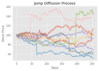
plt.plot(j)
plt.xlabel('Days')
plt.ylabel('Stock Price')
plt.title('Jump Diffusion Process')
Without going into any particular mathematics or demonstrations, we can assert here that the price for options that follow a jump diffusion process must always be higher than the standard Black-Scholes formula. Since we are adding randomness (which benefits the option holder), options writers should demand a larger premium for assets that follow a jump diffusion process. Merton makes this point through the fact that these large changes can't be hedged, which will be the subject of a future article.
Closed Form Solution
By closed form here we mean 'not a Monte-Carlo simulation'.
Merton goes on to derive the following solution to price options that follow a jump diffusion process. The summation below takes the Black-Scholes price conditional on knowing exactly how many jumps will occur and weights these values by their corresponding probability under the Poisson distribution. Naturally we will truncate this in the code.
\(V_{MJD}(S,K, T ,r, \sigma , m, v, \lambda) = \displaystyle \sum_{k=0}^{\infty} \frac{exp(-m \ \lambda \ T) (m \ \lambda \ T)^k}{k!} \ V_{BS}(S,K,T, r_n, \sigma_k )\)
The volatility and drift from the formula above, conditional on \(k\) jumps occurring is given below.
\(\sigma_k = \sqrt{ \sigma^2 +k \ \frac{v ^2 }{T} } \\ r_k = r- \lambda(m-1) + \frac{k \ ln(m)}{T}\)
import numpy as np
from scipy.stats import norm
from scipy.optimize import minimize_scalar
N = norm.cdf

def BS_CALL(S, K, T, r, sigma):
    d1 = (np.log(S/K) + (r + sigma**2/2)*T) / (sigma*np.sqrt(T))
    d2 = d1 - sigma * np.sqrt(T)
    return S * N(d1) - K * np.exp(-r*T)* N(d2)

def BS_PUT(S, K, T, r, sigma):
    d1 = (np.log(S/K) + (r + sigma**2/2)*T) / (sigma*np.sqrt(T))
    d2 = d1 - sigma* np.sqrt(T)
    return K*np.exp(-r*T)*N(-d2) - S*N(-d1)


def merton_jump_call(S, K, T, r, sigma, m , v, lam):
    p = 0
    for k in range(40):
        r_k = r - lam*(m-1) + (k*np.log(m) ) / T
        sigma_k = np.sqrt( sigma**2 + (k* v** 2) / T)
        k_fact = np.math.factorial(k)
        p += (np.exp(-m*lam*T) * (m*lam*T)**k / (k_fact))  * BS_CALL(S, K, T, r_k, sigma_k)

    return p


def merton_jump_put(S, K, T, r, sigma, m , v, lam):
    p = 0 # price of option
    for k in range(40):
        r_k = r - lam*(m-1) + (k*np.log(m) ) / T
        sigma_k = np.sqrt( sigma**2 + (k* v** 2) / T)
        k_fact = np.math.factorial(k) #
        p += (np.exp(-m*lam*T) * (m*lam*T)**k / (k_fact)) \
                    * BS_PUT(S, K, T, r_k, sigma_k)
    return p
Let's compare the closed form solution to a Monte-Carlo simulation. Note that we adjust \(m\) to be \(e^{m + \frac{v^2}{2}}\) as shown here so we can compare the numbers we get from the Monte-Carlo and Merton's formula.
For the simulation we use 200,000 paths sampling at once per day over the course of a year, therefore steps = 255.
S = 100 # current stock price
T = 1 # time to maturity
r = 0.02 # risk free rate
m = 0 # meean of jump size
v = 0.3 # standard deviation of jump
lam = 1 # intensity of jump i.e. number of jumps per annum
steps =255 # time steps
Npaths =200000 # number of paths to simulate
sigma = 0.2 # annaul standard deviation , for weiner process
K =100
np.random.seed(3)
j = merton_jump_paths(S, T, r, sigma, lam, m, v, steps, Npaths) #generate jump diffusion paths

mcprice = np.maximum(j[-1]-K,0).mean() * np.exp(-r*T) # calculate value of call

cf_price =  merton_jump_call(S, K, T, r, sigma, np.exp(m+v**2*0.5) , v, lam)

print('Merton Price =', cf_price)
print('Monte Carlo Merton Price =', mcprice)
print('Black Scholes Price =', BS_CALL(S,K,T,r, sigma))

#Merton Price = 14.500570058304778
#Monte Carlo Merton Price = 14.597509592911369
#Black Scholes Price = 8.916037278572539
The results above are acceptably close, in fact we don't actually need to simulate paths for European options, and it would be much faster to just simulate the terminal prices, but perhaps having the code like this will be useful for future posts on pricing exotic options. Since there is a closed form method we won't worry about this too much. Notice how much of an increase in the price of the call option when we assume the asset follows a jump diffusion process!
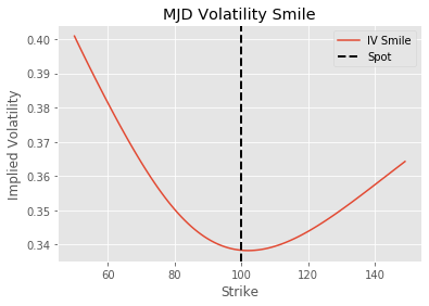
Volatility Smile from Merton's Model
Below we create artificial data and investigate if the model produces a volatility smile using artificial data and the closed form solution. To run this script you will need the Black-Scholes and Implied Volatility scripts from previous articles. Note here that we use the definition of m from Wolfram's article linked above. Therefore when m =1 the mean is zero.
S = 100
strikes = np.arange(50,150,1)
r = 0.02
m = 1
v = 0.3
lam =1
sigma = 0.2
T= 1

mjd_prices = merton_jump_call(S, strikes, T, r, sigma, m, v, lam)
merton_ivs = [implied_vol(c, S, k, T, r) for c,k in zip(mjd_prices, strikes)]

plt.plot(strikes, merton_ivs, label='IV Smile')
plt.xlabel('Strike')
plt.ylabel('Implied Volatility')
plt.axvline(S, color='black', linestyle='dashed', linewidth=2,label="Spot")
plt.title('MJD Volatility Smile')
plt.legend()
As illustrated below the model does in fact produce a volatility smile. We will leave it to the reader to see how the shape of the IV smile changes when adjusting for \(\lambda , m \ \text{and} \ v\)
Model Calibration to Market Prices
Here we will use least squares to fit the closed form solution discussed above to market data. We can set the problem up as shown below. Where \(V_{mkt}\) is the price of the option observed in the market. In this article we will use the mid point \(\frac{Bid + Ask}{2}\) to fit the line.
\( \underset{\sigma \ \ m \ \ v \ \lambda}{\text{minimize} } \hspace{0.25cm} \displaystyle \sum (V_{mkt} - V_{MJD}(S, K_n, T, r, \sigma, m, v, \lambda))^2 \\ \begin{equation*} \begin{array}{lr@{}c@{}r@{}l} \\ \text{subject to :} & 0 < \sigma <\infty \\ & 0 < m < 2 & \\ & 0 < v < \infty & \\ & 0 \leq \lambda < 5 & \end{array} \end{equation*}\)
The bounds above we came to through reasoning that:
The mean of the jump shouldn't be more/less than +-100%.
The variance is strictly positive.
The number of jumps should be less than 5, this number was half picked at random, half due to the fact that we truncated the summand from the closed form solution to be 40 so it makes sense to pick smaller numbers so that \( \sum_{k=0}^{\infty} \frac{exp(-m \ \lambda \ T) (m \ \lambda \ T)^k}{k!}\) sums to as close to 1 as possible .
These numbers of course could be modified, but on this particular dataset, these parameters provided the best mix of speed and accuracy.
The data used in this section was collected from barchart.com on 8th Jan 2021. You can download this data directly from github or simply use Pandas to download the data directly using the script below. To keep things simple we are only using call options for one expiry. The underlying asset is the S&P500 index.
import pandas as pd
import time
from scipy.optimize import minimize

df = pd.read_csv('https://raw.githubusercontent.com/codearmo/data/master/calls_calib_example.csv')

print(df.head(10))
Here F is the futures price, T is the time to maturity. As mentioned we will be using the Midpoint column to find the optimal parameters.
print(df.head(10))
   Strike  Moneyness     Bid  Midpoint     Ask        F     T
0   900.0       0.76  2856.1   2867.55  2879.0  3803.79  0.74
1  1000.0       0.74  2757.0   2768.45  2779.9  3803.79  0.74
2  1100.0       0.71  2658.0   2669.45  2680.9  3803.79  0.74
3  1200.0       0.68  2559.1   2570.55  2582.0  3803.79  0.74
4  1300.0       0.66  2460.3   2471.75  2483.2  3803.79  0.74
5  1400.0       0.63  2361.6   2373.05  2384.5  3803.79  0.74
6  1500.0       0.61  2263.0   2274.45  2285.9  3803.79  0.74
7  1550.0       0.59  2213.8   2225.25  2236.7  3803.79  0.74
8  1600.0       0.58  2164.7   2176.15  2187.6  3803.79  0.74
9  1650.0       0.57  2115.6   2126.20  2136.8  3803.79  0.74
The optimize is shown below. We are using an initial guess for \(\sigma = 0.15 , \ m = 1, \ v = 0.10 \ \text{and} \ \lambda = 1\).
def optimal_params(x, mkt_prices, strikes):
    candidate_prices = merton_jump_call(S, strikes, T, r,
                                        sigma=x[0], m= x[1] ,
                                        v=x[2],lam= x[3])
    return np.linalg.norm(mkt_prices - candidate_prices, 2)


T = df['T'].values[0]
S = df.F.values[0]
r = 0
x0 = [0.15, 1, 0.1, 1] # initial guess for algorithm
bounds = ((0.01, np.inf) , (0.01, 2), (1e-5, np.inf) , (0, 5)) #bounds as described above
strikes = df.Strike.values
prices = df.Midpoint.values

res = minimize(optimal_params, method='SLSQP',  x0=x0, args=(prices, strikes),
                  bounds = bounds, tol=1e-20,
                  options={"maxiter":1000})
sigt = res.x[0]
mt = res.x[1]
vt = res.x[2]
lamt = res.x[3]

print('Calibrated Volatlity = ', sigt)
print('Calibrated Jump Mean = ', mt)
print('Calibrated Jump Std = ', vt)
print('Calibrated intensity = ', lamt)

#Calibrated Volatlity =  0.06489478237064618
#Calibrated Jump Mean =  0.8789051095314648
#Calibrated Jump Std =  0.1542041201811455
#Calibrated intensity =  0.9722952134238365
The optimal parameters are as follows
\(\sigma^* = 0.065 , \ m^* = 0.88, \ v^* = 0.15 \ \text{and} \ \lambda^* = 0.97\)
These numbers do look a little weird, as the volatility seems way too small. Perhaps things would become more realistic if we were to use the entire chain for all expirations. The jump mean, std and intensity look reasonable though.
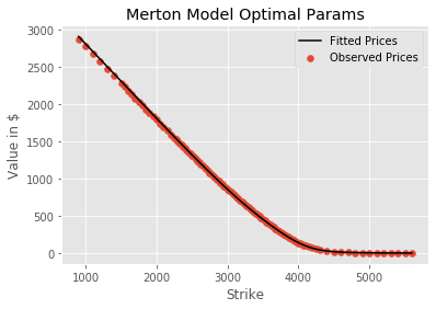
Now that we have these optimal parameters we can reprice the options and plot the fitted values and the observed prices.
df['least_sq_V'] = merton_jump_call(S, df.Strike, df['T'], 0 ,sigt, mt, vt, lamt)

plt.scatter(df.Strike, df.Midpoint,label= 'Observed Prices')
plt.plot(df.Strike, df.least_sq_V, color='black',label= 'Fitted Prices')
plt.legend()
plt.xlabel('Strike')
plt.ylabel('Value in $')
plt.title('Merton Model Optimal Params')
It may not be clear why we would want to find these optimal parameters, but consider pricing a path dependent option on an asset that follows a jump diffusion process. Since we would need to simulate paths to price such an option, we could use this method to find which parameters to feed into the model.