In this article we will cover some advanced options trading strategies that involve buying and selling a mix of both calls and puts options. The code for recreating the diagrams used for this article can be found at the end of the document. In the interests of simplicity we will assume that we only buy a single option, whereas in real life options contracts generally come in lots of 100.
Straddle Strategy
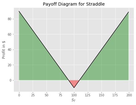
A straddle is a strategy in which a trader buys both a call option and a put option at the same strike price. The idea here is that the trader will benefit from a large move in the price of the underlying stock regardless of the direction of the move. This is an especially useful strategy when a trader predicts a large increase in the uncertainty of an asset price, and the likelihood of a large move, but he is unsure about the direction of the move. For example, say XYZ company earnings are going to be released in the next week, a trader could buy a straddle expecting the company to blow past earnings estimates or dramatically under perform, since we aren't sure about which of the two scenarios will happen, we can buy both a put and a call.
Since we are buying a call option, the potential profit from entering this strategy is potentially unlimited, however, since we are also buying a put option the cost of entering a strategy such as this is higher than just buying one or the other.
Let's take an example of a straddle strategy. Say XYZ companies earnings are coming out next week, you observe a call and a put option in the market selling for $5 each at a strike price of $100 and the stock is currently trading at $100 also.
obj = OptionStrat('Straddle', 100)
obj.long_put(100,5)
obj.long_call(100, 5)
obj.plot(color='black')
We can also implement a short straddle position if we believe the stock will stay around the area it is currently. Going back to the example of XYZ company, perhaps we take the view that the earnings will be exactly as expected and therefore the news is already priced into the stock, we could sell both a call and a put option to collect the premiums with the view that the stock will be around its current level this time next week.
obj = OptionStrat('Short Straddle', 100)
obj.short_put(100,5)
obj.short_call(100, 5)
obj.plot(color='black')

Clearly there is much more downside risk associated with a short straddle strategy. Below we will examine another possible strategy if we take the view that the stock will stay approximately at its current levels.
Butterfly Strategy
As we mentioned for the reverse straddle strategy, the downside is potentially unlimited for entering this position. Say a trader wants to target the same area of the curve, but wants to limit his downside, a butterfly spread strategy is a good option in this case. The strategy makes money if the underlying stock price stays around its current level. To enter into a butterfly strategy we should buy one deep in-the-money call and one out of the money call, to balance the long call positions, we would sell 2 options at the same strike. Recall the discussion on a short straddle, where the trader takes the view that the underlying price will be approximately at the same level it is is now, the butterfly strategy is perhaps a better option as the payoff is realized should the trader's view is correct, with a limited downside should the stock move strongly in either direction.
Lets take an example to show how butterfly strategies can be implemented.
A stock is selling at $100 currently and a trader want to take a position on the price of the stock in 1 month will be approximately where it is now ($100).
Option 1: BUY a call option with strike price $94 for $8
Option 2: BUY a call option with a strike price $106 for $2
Option 3: SELL TWO call options with a strike price of $100 for $4 each for a total of $8.
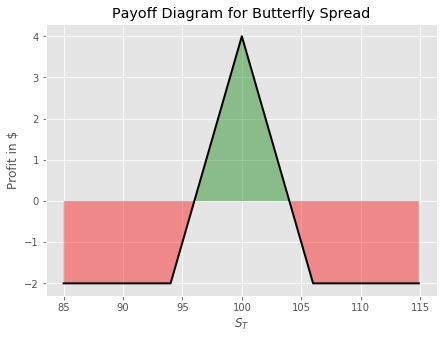
Putting these numbers into the Python script, we can plot and describe the the maximum profit and loss that can be gained from this strategy.
obj = OptionStrat('Butterfly Spread', 100, {'start': 85, 'stop':115,'by':0.1})
obj.long_call(94, 8, 1)
obj.long_call(106, 2, 1)
obj.short_call(100, 4, 2)
obj.plot(color='black', linewidth=2)
obj.describe()

#
#Max Profit: $4.0
#Max loss: $-2.0
#Option(type=call,K=94, price=8,side=long)
#Option(type=call,K=106, price=2,side=long)
#Option(type=call,K=100, price=4,side=short)
#Option(type=call,K=100, price=4,side=short)
#Cost of entering position $2
Notice on the plot below that the maximum profit is realized if the stock price at expiration is equal to the strike of the two calls we shorted when entering the position. This may be a better option than the short straddle if we wanted to take the view that the price of the stock will be similar to its current levels, since the downside is limited.
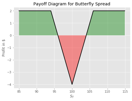
Of course we can also take a short butterfly position. This position can be taken if we wanted to take the view that the stock is likely to move away from its current level but we also want to have reduced downside.
obj = OptionStrat('Butterfly Spread', 100, {'start': 85, 'stop':115,'by':0.1})
obj.short_call(94, 8, 1)
obj.short_call(106, 2, 1)
obj.long_call(100, 4, 2)
obj.plot(color='black', linewidth=2)
obj.describe()
Strangle Strategy
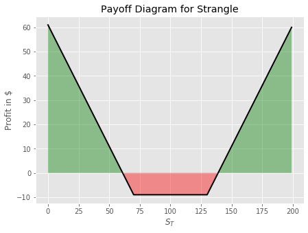
A strangle strategy is similar to a straddle in that the trader wants to take a position that will profit from a large change in the underlying stock price. The difference between a strangle and a straddle is that with a strangle the strike prices of the two options are different whereas in a straddle they are the same. To enter a strangle is cheaper than a straddle, but the stock will need to move further in order for the trader to realize a profit.
An example of a strangle strategy is given below.
Consider a stock that is currently trading at $100 per share, you observe two options in the market.
Option 1: A call option for $4 with a strike at $130
Option 2: A put option for $5 with a strike at $70
To enter into a strangle you would buy both these options. For this strategy to make money the stock must be less than $61 or greater than $139. This is due to the fact that the cost of entering the strategy is $9 and to make money we need to be above/below either strike at expiration plus the cost of entry.
obj = OptionStrat('Strangle', 100)
obj.long_call(130, 4, 1)
obj.long_put(70, 5, 1)
obj.plot(color='black', linewidth=2)
obj.describe()
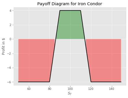
Iron Condor Strategy
An Iron Condor strategy involves buying both a bull put spread and a bear call spread simultaneously, this is similar to a butterfly strategy except the returns are more spread out and the maximum profit is realized at a range of stock prices at expiration. There is also limited downside should the stock make a large move in either direction.
It may be useful to refresh on what bull and bear spreads are, read this article for a refresher.
An example of an Iron Condor is given below. Assume that stock is currently trading at $100
Bull Put Spread.
Option 1: SELL a put with a strike of $90 for $4.
Option 2: BUY a put with a strike of $80 for $2
Bear Call Spread
Option 3: SELL a call with a strike price of $110 for $4.
Option 4: BUY a call with a strike price of $120 for $2.
Let's put those numbers into Python and plot the resulting payoff diagram
obj = OptionStrat('Iron Condor', 100, {'start': 50, 'stop':150,'by':1})
obj.long_call(120, 2, 1)
obj.short_call(110, 4, 1)
obj.short_put(90, 4, 1)
obj.long_put(80, 2, 1)
obj.plot(color='black', linewidth=2)
obj.describe()
Notice that we max a profit as long as the stock stays within a range around the current stock price. With limited downside if the stock experiences a large move in either direction.
Custom Strategy
Of course traders are not limited to these set strategies and they can create their own to target different ranges of stock prices at expiration. Below we give an example of buying and selling both calls and puts and show the resulting payoff diagram.
obj = OptionStrat('Custom', 100)
obj.long_call(120,2, 1)
obj.long_call(100,4 , 7)
obj.short_call(150,0.75,3)
obj.long_put(80, 2, 4)
obj.short_put(40, 0.65, 10)
obj.plot(color='black')
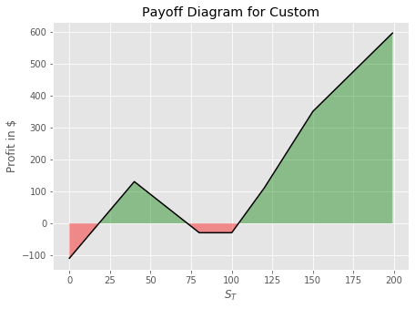
Perhaps you can try to add different positions and view the resulting diagram, it is good fun!
The Python code to recreate the diagrams is given below.
class Option:
    def __init__(self, type_, K, price, side):
        self.type = type_
        self.K = K
        self.price = price
        self.side = side

    def __repr__(self):
        side = 'long' if self.side == 1 else 'short'
        return f'Option(type={self.type},K={self.K}, price={self.price},side={side})'

class OptionStrat:
    def __init__(self, name, S0, params=None):
        self.name = name
        self.S0 = S0
        if params:
            self.STs=np.arange(params.get('start',0),
                               params.get('stop', S0*2), params.get('by',1))
        else:
            self.STs = np.arange(0, S0*2, 1)
        self.payoffs = np.zeros_like(self.STs)
        self.instruments = []

    def long_call(self, K, C, Q=1):

        payoffs =  np.array([max(s-K,0)  - C for s in self.STs])*Q
        self.payoffs = self.payoffs +payoffs
        self._add_to_self('call', K, C, 1, Q)

    def short_call(self, K, C, Q=1):
        payoffs =  np.array([max(s-K,0) * -1 + C for s in self.STs])*Q
        self.payoffs = self.payoffs + payoffs
        self._add_to_self('call', K, C, -1, Q)

    def long_put(self, K, P, Q=1):
        payoffs = np.array([max(K-s,0) - P for s in self.STs])*Q
        self.payoffs = self.payoffs + payoffs
        self._add_to_self('put', K, P, 1, Q)

    def short_put(self, K, P, Q=1):
        payoffs = np.array([max(K-s,0)*-1 + P for s in self.STs])*Q
        self.payoffs = self.payoffs + payoffs
        self._add_to_self('put', K, P, -1, Q)

    def _add_to_self(self, type_, K, price, side, Q):
        o = Option(type_, K, price, side)
        for _ in range(Q):
            self.instruments.append(o)


    def plot(self, **params):
        plt.plot(self.STs, self.payoffs,**params)
        plt.title(f"Payoff Diagram for {self.name}")
        plt.fill_between(self.STs, self.payoffs,
                         where=(self.payoffs >= 0), facecolor='g', alpha=0.4)
        plt.fill_between(self.STs, self.payoffs,
                         where=(self.payoffs < 0), facecolor='r', alpha=0.4)

        plt.xlabel(r'$S_T$')
        plt.ylabel('Profit in $')
        plt.show()

    def describe(self):
        max_profit  = self.payoffs.max()
        max_loss = self.payoffs.min()
        print(f"Max Profit: ${round(max_profit,3)}")
        print(f"Max loss: ${round(max_loss,3)}")
        c = 0
        for o in self.instruments:
            print(o)
            if o.type == 'call' and o.side==1:
                c += o.price
            elif o.type == 'call' and o.side == -1:
                c -= o.price
            elif o.type =='put' and o.side == 1:
                c += o.price
            elif o.type =='put' and o.side == -1:
                c -+ o.price

        print(f"Cost of entering position ${c}")