Calculating the Volatility Smile

 

The volatility smile is related to the fact that options at different strikes have different levels of implied volatility. Since volatility is the only parameter which is unobserved (in Black-Scholes) it is an important concept to grasp. In this article we will calculate the implied volatility for options at different strikes using Scipy. To see a from scratch implementation of calculating implied volatility using Newton's method see here. 

 

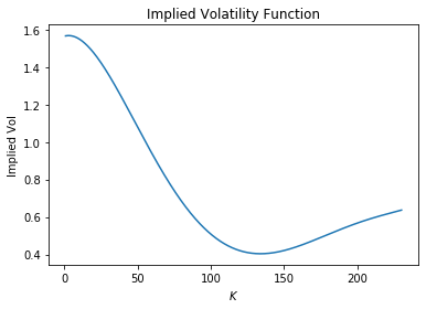
In the article on binary options we observed from market data that the volatility is not constant from market prices and this implies a heavier tail probability that the log-normal distribution that the Black-Scholes model assumes. The plot below is the implied volatility curve for Apple options as discussed in the article on binaries. 

 

 

We can look at calculating implied volatility as a minimize problem. Below we minimize the absolute difference between the market price and the Black-Scholes price. We have bounded this minimization such that the volatility is less than 600%. This number was chosen without much thought, so feel free to change it or let me know if it should be higher/lower. 

 

Let \(V\) below be the value of a European call or put option. 

 

\(\text{implied volatility} = \underset{\sigma{\in(0, 6]}}{\arg\min} \ |V_{market} - V_{BS}(S,K, T, r ,\sigma)|\)

 

 

To complete the logic above we will use Scipy's minimize_scalar function which uses Brent's method underneath the hood. This method seems to be more robust than the Newton implementation  shown previously. This is perhaps due to that fact that vega will be close to zero for out of the money options. 

 

The Black-Scholes functions BS_CALL and BS_PUT are explained here. 

 

import numpy as np
from scipy.stats import norm
from scipy.optimize import minimize_scalar   
import pandas as pd
import pandas_datareader.data as web
import datetime as dt
N = norm.cdf

def BS_CALL(S, K, T, r, sigma):
    d1 = (np.log(S/K) + (r + sigma**2/2)*T) / (sigma*np.sqrt(T))
    d2 = d1 - sigma * np.sqrt(T)
    return S * N(d1) - K * np.exp(-r*T)* N(d2)

def BS_PUT(S, K, T, r, sigma):
    d1 = (np.log(S/K) + (r + sigma**2/2)*T) / (sigma*np.sqrt(T))
    d2 = d1 - sigma* np.sqrt(T)
    return K*np.exp(-r*T)*N(-d2) - S*N(-d1)    
    

def implied_vol(opt_value, S, K, T, r, type_='call'):
    
    def call_obj(sigma):
        return abs(BS_CALL(S, K, T, r, sigma) - opt_value)
    
    def put_obj(sigma):
        return abs(BS_PUT(S, K, T, r, sigma) - opt_value)
    
    if type_ == 'call':
        res = minimize_scalar(call_obj, bounds=(0.01,6), method='bounded')
        return res.x
    elif type_ == 'put':
        res = minimize_scalar(put_obj, bounds=(0.01,6),
                              method='bounded')
        return res.x
    else:
        raise ValueError("type_ must be 'put' or 'call'")
        

 

The small example below tests that the implied volatility function calculates things as expected. This function is quite fast which is good and it seems to work correctly. 

 

###testing implied vol function####
S = 100
K = 100
T = 1
r = 0.05
sigma = 0.45

C = BS_CALL(S, K, T, r, sigma)
iv = implied_vol(C, S, K, T, r)
print(iv)

#0.45000020780432554

 

 

Let's try calculating the implied volatility for Tesla options. Luckily Yahoo Finance provides a estimate of implied volatility also so we have something to benchmark on. For simplicity we assume interests rates are zero. This isn't such a big deal since at the time of writing interests rates are as close to zero as is possible. I have found the calculated volatility to be more accurate when using the ask price from Yahoo Finance, but feel free to check the bid or the mid also. 

 

The data you receive when you run this script will be different as this was called on the 04/01/2021, but you should observe a similar shape to the smile. 

 

tsla = web.YahooOptions('TSLA')
calls = tsla.get_call_data()

calls.reset_index(inplace=True)
calls['mid'] = (calls.Bid + calls.Ask)/2
calls['Time'] = (calls.Expiry - dt.datetime.now()).dt.days / 255


ivs = [] 

for row in calls.itertuples():
    iv = implied_vol(row.Ask, row.Underlying_Price, row.Strike, row.Time, 0.00)
    ivs.append(iv)


plt.scatter(calls.Strike, ivs, label='calculated')
plt.scatter(calls.Strike, calls.IV, label='Provided')
plt.xlabel('Strike')
plt.ylabel('Implied Vol')
plt.title('Implied Volatility Curve for Facebook')
plt.legend() 

 

 

 

 

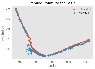
It looks like we have replicated the implied volatilities quite accurately, perhaps the error arises due to a combination of the fact that we assumed interests rates are 0 and we also only considered the ask price for the minimization problem. Feel free to try out other stocks to see what sort of curve you get!