In this article we will discuss a number of common strategies that speculators will enter with the intention to make profit. The code to recreate the plots and create your own is provided at the end of the document.
Bull Call Spread
A bull call spread is a strategy in which a trader buys one call option and sells (writes) another. This strategy should be used when the trader believes the stock will increase in value.
This strategy has a cap on the potential profit, the maximum profit is as follows.
\((K_1 - K_2) - (C_2 - C_1) \hspace{0.25cm}\text{where} \ K_1 > K_2\)
\(K = \text{strike} , C = \text{call price} \)
The maximum loss is as follows:
\(C_1 - C_2\)
Let's take a quick example.
Option 1 C1: This option has a strike price of $130 and is currently selling at $5
Option 2 C2: This option has a strike price of $90 and is currently selling for $20
The maximum profit in this case is \((K_1 - K_2) - (C_2 - C_1) = (130-90) - (20-5) = $25\)
The maximum loss in this case \(C_1 - C_2 = 5 - 20 = -$15\)
obj = OptionStrat('Bull Call Spread', 100)
obj.short_call(130, 5)
obj.long_call(90, 20)
obj.plot(color='black')
obj.describe()

#Max Profit: $25
#Max loss: $-15
#Option(type=call,K=130, price=5,side=short)
#Option(type=call,K=90, price=20,side=long)
#Cost of entering position $15
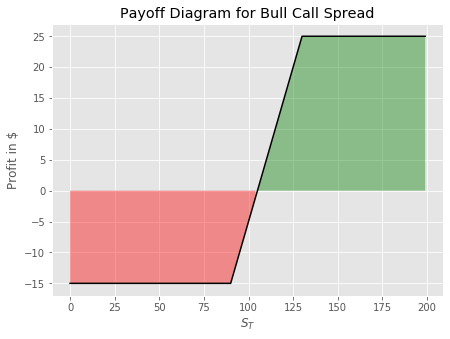
Notice on the diagram below that for higher future stock prices on the expiration date the position shows a profit up to a maximum of $25 and for lower \(S_T\) values the position loses money to a maximum loss of $15.
Bear Call Spread
A bear call spread is the opposite of a bull spread, in this strategy we sell a call option with a lower strike and buy another with a higher strike. This strategy is useful when a trader expects the price of the stock to go down.
\((C_1 - C_2), \hspace{0.3cm} \text{where} \hspace{0.3cm} C_1 > C_2\)
The maximum loss from this strategy is
\((K_1 - K_2) + (C_1 - C_2)\)
Let's take a specific example to put a bear call spread into context.
Option 1: Call option selling for $2.50 at a strike price of $30.
Option 2: Call option selling for $0.5 at a strike price of $35.
To enter a bear call spread, we would sell option 1 and receive an inflow of $2.50 and buy option 2 for $0.50. The total inflow from this position is +$2.00. The maximum profit is $2.50 - $0.5 = $2.00 and the maximum loss is \((K_1 - K_2) + (C_1 - C_2) = (30 - 35) + (2.50 -0.50) = -$3.00\)
The example above is put into the OptionStrat object below, assume that the current price is $30.
obj = OptionStrat('Bear Call Spread', 30)
obj.short_call(30,2.50)
obj.long_call(35, 0.5)
obj.plot(color='black')
obj.describe()

#Max Profit: $2.0
#Max loss: $-3.0
#Option(type=call,K=30, price=2.5,side=short)
#Option(type=call,K=35, price=0.5,side=long)
#Cost of entering position $-2.0
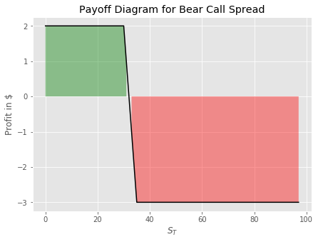
This script will return the diagram depicted below. The green section is limited to a maximum of $2 and the red section is limited to a maximum loss of $3.00 as we seen above.
Bull Put Spread
A bull spread using puts can also be constructed. Again this is a strategy we would implement if we took the view that the price of the stock will go up, whilst also limiting our downside. Since we expect the price to go up, we will sell a put option with a higher strike (more valuable at time \(T_0\)) and buy another with a lower strike price, the lower strike we buy acts as a way to limit our losses should the stock move against us.
Maximum profit from bull spread with puts. Is the net inflow received from selling one put option and buying another.
\(C_1 - C_2 \hspace{0.25cm} where \ C_1 > C_2\)
Maximum loss from entering this position.
\(-(K_1- K_2) + (C_1 - C_2)\)
Let's take an example to put this into context.
Option 1: There is an option selling for $15 with a strike of $110, assume that the stock is currently trading at $100
Option 2: There is an option selling for $4 with a strike of $90.
So we would sell option 1 and buy option 2 to enter into a bull put spread.
The maximum profit in this case would be \(C_1 - C_2 = (15 - 4) = $11\)
The maximum loss in this case would be \(-(K_1- K_2) + (C_1 - C_2) = -(110 - 90) + (15 -4) = -$9\)
obj = OptionStrat('Bull Put Spread', 100)
obj.long_put(90,4)
obj.short_put(110, 15)
obj.plot(color='black')
obj.describe()

#Max Profit: $11
#Max loss: $-9
#Option(type=put,K=90, price=4,side=long)
#Option(type=put,K=110, price=15,side=short)
#Cost of entering position $4
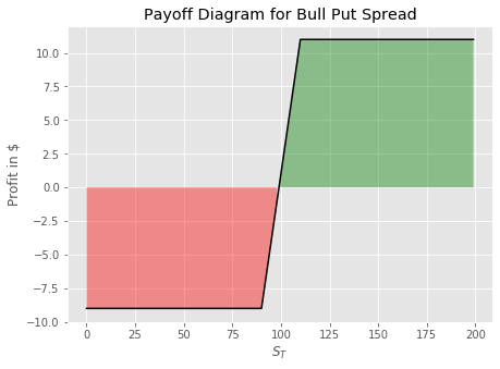
As we see from the diagram below, the strategy returns a profit up to a maximum of $11 on higher values of the stock price and limits our losses to a maximum of $9.
Bear Put Spread
A bear put spread can be implemented if the trader wants to take a position on the stock decreasing in value. In order to take this position we need to sell one put option with a lower strike price and buy another with a higher strike price. This is a good way to bet against a stock whilst also having limited downside.
Maximum profit from bull spread with puts. Is the net inflow received from selling one put option and buying another.
\((K_1 - K_2) - (C_1 - C_2) \hspace{0.25cm} where \hspace{0.25cm} K_1 > K_2\)
Maximum loss from entering this position.
\(- (C_1 - C_2)\)
Let's take an example to put a bear spread into context.
Option 1: There is a put option selling for $3 with a strike of $90 for a stock that is currently priced at $100.
Option 2: There is another put option selling for $1 with a strike of $80.
To implement a bear put spread we would buy option 1 and sell option 2.
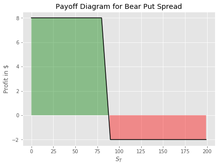
Maximum profit in this case is \((K_1 - K_2) - (C_1 - C_2) = (90 - 80) - (3-1) = $8\)
Maximum loss in this case is \(- (C_1 - C_2) = -(3-1) = -$2\)
obj = OptionStrat('Bear Put Spread', 100)
obj.long_put(90,3)
obj.short_put(80,1)
obj.plot(color='black')
obj.describe()

#Max Profit: $8
#Max loss: $-2
#Option(type=put,K=90, price=3,side=long)
#Option(type=put,K=80, price=1,side=short)
#Cost of entering position $3
It may be worth playing around with the code here to try out different strikes for each of the 4 strategies we discussed here. See if you can figure out the relationship between the distance between strikes and the potential for profit and loss for each of the strategies.
class Option:
    def __init__(self, type_, K, price, side):
        self.type = type_
        self.K = K
        self.price = price
        self.side = side

    def __repr__(self):
        side = 'long' if self.side == 1 else 'short'
        return f'Option(type={self.type},K={self.K}, price={self.price},side={side})'

class OptionStrat:
    def __init__(self, name, S0):
        self.name = name
        self.S0 = S0
        self.STs = np.arange(0, S0*2, 1)
        self.payoffs = np.zeros_like(self.STs)
        self.instruments = []

    def long_call(self, K, C, Q=1):

        payoffs =  np.array([max(s-K,0)  - C for s in self.STs])*Q
        self.payoffs = self.payoffs +payoffs
        self._add_to_self('call', K, C, 1, Q)

    def short_call(self, K, C, Q=1):
        payoffs =  np.array([max(s-K,0) * -1 + C for s in self.STs])*Q
        self.payoffs = self.payoffs + payoffs
        self._add_to_self('call', K, C, -1, Q)

    def long_put(self, K, P, Q=1):
        payoffs = np.array([max(K-s,0) - P for s in self.STs])*Q
        self.payoffs = self.payoffs + payoffs
        self._add_to_self('put', K, P, 1, Q)

    def short_put(self, K, P, Q=1):
        payoffs = np.array([max(K-s,0)*-1 + P for s in self.STs])*Q
        self.payoffs = self.payoffs + payoffs
        self._add_to_self('put', K, P, -1, Q)

    def _add_to_self(self, type_, K, price, side, Q):
        o = Option(type_, K, price, side)
        for _ in range(Q):
            self.instruments.append(o)


    def plot(self, **params):
        plt.plot(self.STs, self.payoffs,**params)
        plt.title(f"Payoff Diagram for {self.name}")
        plt.fill_between(self.STs, self.payoffs,
                         where=(self.payoffs > 0), facecolor='g', alpha=0.4)
        plt.fill_between(self.STs, self.payoffs,
                         where=(self.payoffs < 0), facecolor='r', alpha=0.4)

        plt.xlabel(r'$S_T$')
        plt.ylabel('Profit in $')
        plt.show()

    def describe(self):
        max_profit  = self.payoffs.max()
        max_loss = self.payoffs.min()
        print(f"Max Profit: ${round(max_profit,3)}")
        print(f"Max loss: ${round(max_loss,3)}")
        c = 0
        for o in self.instruments:
            print(o)
            if o.type == 'call' and o.side==1:
                c += o.price
            elif o.type == 'call' and o.side == -1:
                c -= o.price
            elif o.type =='put' and o.side == 1:
                c += o.price
            elif o.type =='put' and o.side == -1:
                c -+ o.price

        print(f"Cost of entering position ${c}")