In this article we will consider the first-order sensitivities for options under a Black-Scholes framework. There are 5 important sensitivities to consider when pricing options. We will explore before numerical methods and analytic solutions to calculate these values. The values discussed in this article are useful for option trading to measure the risk of their options portfolio.
Contents
- Finite Differences Intro
- Delta
- Gamma
- Vega
- Theta
-Rho
Math Refresher
Consider the formula before for the definition of a derivative for a single variable function that should be familiar.
\(f'(x) = \lim\limits_{h \rightarrow 0} \frac{f(x+h) - f(x)}{h} \)
Let's take a super simple example to examine how finite differences work.
\(f(x) = e^x\)
Clearly we know that the derivative \(f'(x) = e^x\) in this case as it is with all the higher order derivatives, it is for this reason we will use it as an example to show how we can calculate the derivative as a finite difference.
Forward Difference
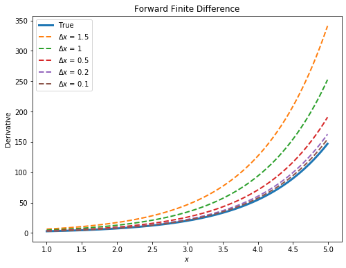
We will rewrite the definition of a derivative above, to keep with the convention that \(h\ \text{becomes} \ \Delta x\). Where as before \(h\) is some infinitesimally small number, \(\Delta x\) is now some finite positive number. Note that \(O(\Delta x)\) is a constant which you can think of as the error, by decreasing \(\Delta x\) this number reduces as we get a more accurate approximation. We won't cover in depth where this comes from but this wiki is very good should you wish to learn more.
\(f'(x) = \frac{f(x+\Delta x) - f(x)}{\Delta x} + O(\Delta x)\)
Let's make a forward difference function in Python and try it out on \(f(x) = e^x\) to gain some intuition about how it all works.
def f(x):
    return np.exp(x)

def forward_difference(f, x, dx):
    return (f(x+dx) - f(x)) / dx

plt.figure(figsize=(8, 6))
deltasxs = [1.5, 1, 0.5, 0.2, 0.1]
nums = np.arange(1,5,0.01)

plt.plot(nums, true, label= 'True',linewidth=3)
for delt in deltasxs:
    plt.plot(nums, forward_difference(f, nums, delt), label=f'$\Delta x$ = {delt}',linewidth=2,linestyle='--')

plt.legend()
plt.ylabel("Derivative")
plt.xlabel('$x$')
plt.title('Forward Finite Difference')
For the second derivative \(f''(x)\) we are approximating the change of the first derivative for a small change in x therefore the formula is as follows;
\(f''(x) = \frac{ \frac{f(x+2\Delta x) - f(x - \Delta x)}{\Delta x} - \frac{f(x+\Delta x) - f(x)} {\Delta x} }{\Delta x} = \frac{ f(x+2\Delta x) -2f(x +\Delta x)+ f(x)}{(\Delta x )^2}\)
We will leave the Python coding for this as an exercise to the reader, as we will be showing how to do this later on in the document in an applied sense.
Backward Difference
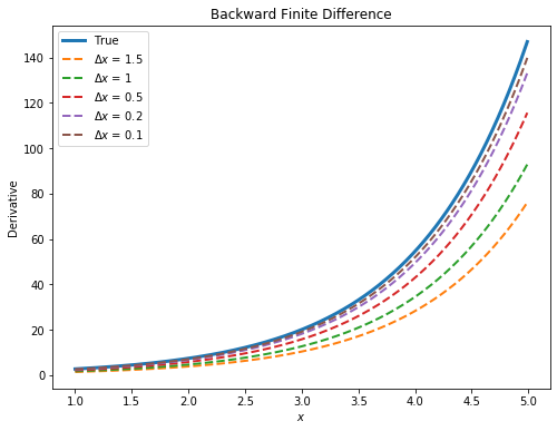
We can also calculate a backwards difference, this is done by taking a finite step backwards on the function and seeing how much it has changed from the current value
\(f'(x) = \frac{f(x) - f(x-\Delta x) }{\Delta x} + O(\Delta x)\)
def backward_difference(f, x, dx):
    return (f(x) - f(x-dx)) / dx

nums = np.arange(1,5,0.01)
true = f(nums)
plt.figure(figsize=(8, 6))
deltasxs = [1.5, 1, 0.5, 0.2, 0.1]

#plt.plot(nums, f(nums))
plt.plot(nums, true, label= 'True',linewidth=3)
for delt in deltasxs:
    plt.plot(nums, backward_difference(f, nums, delt),
             label=f'$\Delta x$ = {delt}',
             linewidth=2, linestyle='--')

plt.legend()
plt.ylabel("Derivative")
plt.xlabel('$x$')
plt.title('Backward Finite Difference')
Again we can calculate the 2nd derivative as shown below.
\(f''(x) = \frac{ \frac{f(x) - f(x - \Delta x)}{\Delta x} - \frac{f(x-\Delta x) - f(x -2\Delta x)} {\Delta x} }{\Delta x} = \frac{ f(x) -2f(x -\Delta x)+ f(x - 2\Delta x)}{(\Delta x )^2}\)
Central Difference
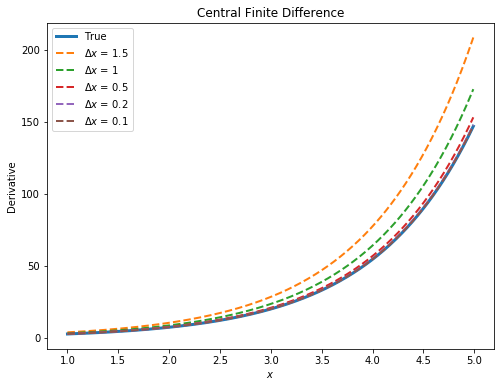
A central difference combines both the forward and backward difference methods explained above and takes an average of the two. This is known as a second order finite difference, it shouldn't be surprising that this will be a more accurate approximation.
\(f'(x) = \frac{f(x+ \Delta x) -f(x-\Delta x) }{2\Delta x} + O(\Delta x)^2\)
def central_difference(f, x, dx):
    return (f(x+dx) - f(x-dx)) / (2*dx)


plt.figure(figsize=(8, 6))
deltasxs = [1.5, 1, 0.5, 0.2, 0.1]

#plt.plot(nums, f(nums))
plt.plot(nums, true, label= 'True',linewidth=3)
for delt in deltasxs:
    plt.plot(nums, central_difference(f, nums, delt), label=f'$\Delta x$ = {delt}',linewidth=2,linestyle='--')

plt.legend()
plt.ylabel("Derivative")
plt.xlabel('$x$')
plt.title('Central Finite Difference')
\(f''(x) = \frac{ \frac{f(x+\Delta x ) - f(x )}{\Delta x} - \frac{f(x) - f(x -\Delta x)} {\Delta x} }{\Delta x} = \frac{ f(x +\Delta x ) -2f(x)+ f(x -\Delta x)}{(\Delta x )^2}\)
For the remainder of this article we will use the Black-Scholes call and put formulas from this article on the subject.
Delta Analytic
Delta is simply the ratio of a change in the price of an option relative to a change in the price of the underlying. Think of delta intuitively as speed, in that it measures the speed of change in the option for a change in the underlying.
\(\frac{\partial C}{\partial S} = N(d_1) \hspace{0.5cm} \frac{\partial P}{\partial S} = -N(-d_1)\)
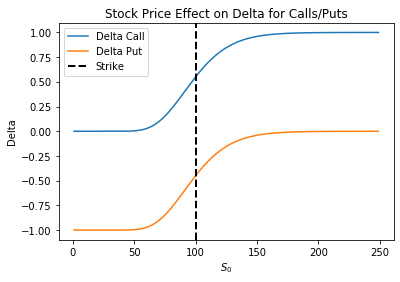
The delta of an option will be between [0,1] for a call option and [-1, 0] for a put option. This should make sense in that a put option moves inversely to the price of the underlying, where a call option moves in the same direction.
Example
A stock is currently $100 and you have an options portfolio with two options.
Option 1 has a delta of 0.5 and you own 10 contracts of 100 options per contract
Option 2 has a delta of 0.2 and you are short 5 contracts of 100 options per contract.
Let's consider a two scenarios.
Scenario 1: Stock increases by $1
\(\text{Change in dollars}= delta \times \text{number of contracts} \times \text{change in stock price}\)
The formula above is how we calculate the change in the position.
Resulting change in option 1 position is \(0.5 \times 10 \times 100 \times 1 = + $500 \)
Resulting change in option 2 position is \(-0.2 \times 5 \times 100 \times 1 = - $100 \)
Total change in portfolio is then +$400. Notice here that the sign on the delta is reversed since we are short the option.
Scenario 2 Stock decreases by $0.5
Resulting change in option 1 position is \(0.5 \times 10 \times 100 \times -0.5 = - $250 \)
Resulting change in option 2 position is \(-0.2 \times 5\times 100 \times -0.5 =+$50\)
Total change in portfolio is then -$200.
So as we see the delta is additive across different strike prices. As long as the underlying is the same we can add deltas together.
Delta Finite Difference
In the interests of space we will just consider a forward difference, as described in the math section of this article. Although the Python function can use a forward, backward and central difference as shown in the script below. To calculate this simply add a small number to the stock price, the choosing this number as with the math examples at the beginning of the document will have a direct effect on the accuracy.
\(\frac{\partial C}{\partial S} = \frac{BS_{Call}(S+\Delta S, K, T,r,\sigma) - BS_{Call}(S, K, T,r,\sigma)}{\Delta S}\)
Python Implementation.
from scipy.stats import norm
import numpy as np

def d1(S, K, T, r, sigma):
    return (np.log(S/K) + (r + sigma**2/2)*T) /\
                     (sigma*np.sqrt(T))

def d2(S, K, T, r, sigma):
    return d1(S, K, T, r, sigma) - sigma* np.sqrt(T)

def delta_call(S, K, T, r, sigma):
    N = norm.cdf
    return N(d1(S, K, T, r, sigma))

def delta_fdm_call(S, K, T, r, sigma, ds = 1e-5, method='central'):
    method = method.lower()
    if method =='central':
        return (BS_CALL(S+ds, K, T, r, sigma) -BS_CALL(S-ds, K, T, r, sigma))/\
                        (2*ds)
    elif method == 'forward':
        return (BS_CALL(S+ds, K, T, r, sigma) - BS_CALL(S, K, T, r, sigma))/ds
    elif method == 'backward':
        return (BS_CALL(S, K, T, r, sigma) - BS_CALL(S-ds, K, T, r, sigma))/ds


def delta_put(S, K, T, r, sigma):
    return - N(-d1(S, K, T, r, sigma))

def delta_fdm_put(S, K, T, r, sigma, ds = 1e-5, method='central'):
    method = method.lower()
    if method =='central':
        return (BS_PUT(S+ds, K, T, r, sigma) -BS_PUT(S-ds, K, T, r, sigma))/\
                        (2*ds)
    elif method == 'forward':
        return (BS_PUT(S+ds, K, T, r, sigma) - BS_PUT(S, K, T, r, sigma))/ds
    elif method == 'backward':
        return (BS_PUT(S, K, T, r, sigma) - BS_PUT(S-ds, K, T, r, sigma))/ds


S = 100
K = 100
T = 1
r = 0.00
sigma = 0.25

prices = np.arange(1, 250,1)

deltas_c = delta_call(prices, K, T, r, sigma)
deltas_p = delta_put(prices, K, T, r, sigma)
deltas_back_c = delta_fdm_call(prices, K, T,r, sigma, ds = 0.01,method='backward')
deltas_forward_p = delta_fdm_put(prices, K, T,r, sigma, ds = 0.01,method='forward')

plt.plot(prices, deltas_c, label='Delta Call')
plt.plot(prices, deltas_p, label='Delta Put')
plt.xlabel('$S_0$')
plt.ylabel('Delta')
plt.title('Stock Price Effect on Delta for Calls/Puts' )
plt.axvline(K, color='black', linestyle='dashed', linewidth=2,label="Strike")
plt.legend()
Notice that delta changes depending on the stock price. When an option is at the money \(S_0 \approx K\) the delta of a call will be approximately 50% and the delta of a put will be approximately -%50
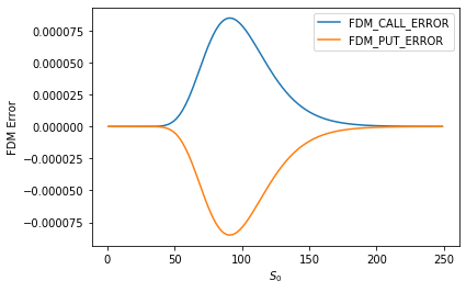
It may also be useful for understanding the next section to view the plot below which shows the error rate for forward and backward finite differences for both calls and puts. Refer to the following article for the call/put prices curve for Black-Scholes and notice that the curvature i.e. the second derivative is greatest near to where the option is in the money. The code below takes the difference between the analytic formula for delta and the finite difference approach.
errorc = np.array(deltas_c) - np.array(deltas_back)
errorp = np.array(deltas_p) - np.array(deltas_forward_p)

plt.plot(prices, errorc, label='FDM_CALL_ERROR')
plt.plot(prices, errorp, label='FDM_PUT_ERROR')
plt.legend()
plt.xlabel('$S_0$')
plt.ylabel('FDM Error')
Therefore the error below is directly proportional to the second derivative known as gamma in the context of equity options.
Gamma Analytic
The formula for gamma is the same for both calls and puts. As shown below.
\(\frac{\partial ^2{C}}{\partial S^2} =\frac{\partial ^2{P}}{\partial S^2} = \frac{N'(d_1)}{S\sigma\sqrt{T}}\)
We gave an intuitive description for delta being the speed in the last section. To understand gamma consider gamma is to acceleration what delta is to speed. So think of a car moving along a road, if we know how fast it is going, we can estimate where the car will be in a certain amount of time. However, this assumes the car is traveling at a constant speed. As the change in speed is known as acceleration, the change in delta is known as gamma.
Gamma Finite Difference
Here we use a central finite difference using the BS_PUT function created in the previous article. As with delta you can change the finite difference method by passing in forward, backward or central into the function.
\(\frac{\partial P}{\partial S} = \frac{BS_{Put}(S+\Delta S, K, T,r,\sigma) - 2BS_{Put}(S,K, T,r,\sigma) +BS_{Put}(S-\Delta S, K, T,r,\sigma)}{(\Delta S)^2}\)
def gamma(S, K, T, r, sigma):
    N_prime = norm.pdf
    return N_prime(d1(S,K, T, r, sigma))/(S*sigma*np.sqrt(T))


def gamma_fdm(S, K, T, r, sigma , ds = 1e-5, method='central'):
    method = method.lower()
    if method =='central':
        return (BS_CALL(S+ds , K, T, r, sigma) -2*BS_CALL(S, K, T, r, sigma) +
                    BS_CALL(S-ds , K, T, r, sigma) )/ (ds)**2
    elif method == 'forward':
        return (BS_CALL(S+2*ds, K, T, r, sigma) - 2*BS_CALL(S+ds, K, T, r, sigma)+
                   BS_CALL(S, K, T, r, sigma) )/ (ds**2)
    elif method == 'backward':
        return (BS_CALL(S, K, T, r, sigma) - 2* BS_CALL(S-ds, K, T, r, sigma)
                + BS_CALL(S-2*ds, K, T, r, sigma)) /  (ds**2)


gammas = gamma(prices, K, T, r, sigma)
gamma_forward = gamma_fdm(prices, K, T, r, sigma, ds =0.01,method='forward')

plt.plot(prices, gammas)
plt.plot(prices, gamma_forward)
plt.title('Gamma by changing $S_0$')
plt.xlabel('$S_0$')
plt.ylabel('Gamma')
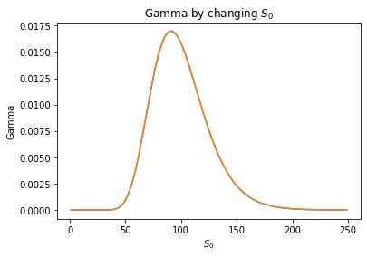
We will leave it to the reader to plot the following and consider what this represents.
plt.plot(gammas -gamma_forward)
Vega Analytic
Vega is the partial derivative of the option with respect to volatility. Refer back to this article to recall how a change in volatility will affect the value of both calls or puts. The plot in the article linked above, shows that the option price is a strictly increasing function of the volatility parameter. Keeping with our car examples, where delta is speed, gamma is acceleration we can think of vega / volatility in general as change in BHP/ BHP.
\(\frac{\partial {C}}{\partial \sigma} =\frac{\partial {P}}{\partial \sigma}=S\sqrt{T} N'(d1)\)
Consider an option that is currently priced at $10 , you calculate the vega as 30 and in the next instant you expect the market to adjust volatility in the security across all strikes by 1% , you would expect the option to increase in value by 30 x %1 = $0.3 , the opposite would be true for a drop of 1%.
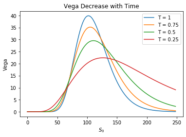
We will now investigate how vega changes as the expiration of the option nears.
Ts = [1,0.75,0.5,0.25]

for t in Ts:
    plt.plot(vega(prices, K, t, r, sigma), label=f'T = {t}')

plt.legend()
plt.xlabel('$S_0$')
plt.ylabel('Vega')
plt.title('Vega Decrease with Time')
Notice that as time to expiration decreases, vega also decreases. Although we may be in danger of slightly abusing our car analogy here, you can roughly think of this as a car in a race nearing the finish line, we are assuming that by some miracle the car can update its brake horsepower (BHP) due to some underlying process throughout a race). As it approaches the finish line, the potential speed of the car matters less and less since there is only a finite amount of time left. So if the car doubled it BHP 100 meters from the finish line the effect on isn't going to be the same as if it had doubled 1000 meters from the finish line (if this is confusing please ignore!!!).
Vega Finite Difference
Here we show calculating vega by using a backward finite difference. The same procedure can be used for puts also.
\(\frac{\partial C}{\partial \sigma} = \frac{BS_{Call}(S, K, T,r,\sigma) - BS_{Call}(S , K, T,r,\sigma -\Delta \sigma )}{\Delta \sigma}\)
def vega(S, K, T, r, sigma):
    N_prime = norm.pdf
    return S*np.sqrt(T)*N_prime(d1(S,K,T,r,sigma))

def vega_fdm(S, K, T, r, sigma, dv=1e-4, method='central'):
    method = method.lower()
    if method =='central':
        return (BS_CALL(S, K, T, r, sigma+dv) -BS_CALL(S, K, T, r, sigma-dv))/\
                        (2*dv)
    elif method == 'forward':
        return (BS_CALL(S, K, T, r, sigma+dv) - BS_CALL(S, K, T, r, sigma))/dv
    elif method == 'backward':
        return (BS_CALL(S, K, T, r, sigma) - BS_CALL(S, K, T, r, sigma-dv))/dv
Theta Analytic
The theta of an option is the also known as the time-decay. It measures the change of the value with respect to time. Both calls and puts will experience a decrease in value as the expiration date nears.
\(\frac{\partial {C}}{\partial T} = -\frac{S \ N'\left ( d1 \right )\sigma}{2\sqrt{T}}-rKe^{-rT}N\left ( d2 \right )\)
\(\frac{\partial {P}}{\partial T} = -\frac{S \ N'\left ( d1 \right )\sigma}{2\sqrt{T}}+rKe^{-rT}N\left ( -d2 \right )\)
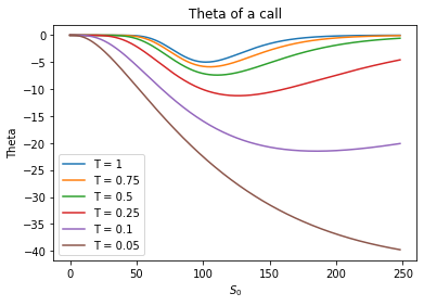
It shouldn't come as a surprise that the theta of a call becomes larger and larger as time to maturity increases. Note that this is for a 1 unit change, so you could multiply this number by 1/255 to get an indication of time decay on a daily basis. We will leave it to the reader to plot a similar graph for the put option.
Theta Finite Difference
Here we use a backward finite difference to calculate theta on a call.
\(\frac{\partial C}{\partial T} = \frac{BS_{Call}(S, K, T +\Delta T,r,\sigma) - BS_{Call}(S, K, T,r,\sigma)}{\Delta T}\)
def theta_call(S, K, T, r, sigma):
    p1 = - S*N_prime(d1(S, K, T, r, sigma))*sigma / (2 * np.sqrt(T))
    p2 = r*K*np.exp(-r*T)*N(d2(S, K, T, r, sigma))
    return p1 - p2

def theta_put(S, K, T, r, sigma):
    p1 = - S*N_prime(d1(S, K, T, r, sigma))*sigma / (2 * np.sqrt(T))
    p2 = r*K*np.exp(-r*T)*N(-d2(S, K, T, r, sigma))
    return p1 + p2

def theta_call_fdm(S, K, T, r, sigma, dt, method='central'):
    method = method.lower()
    if method =='central':
        return -(BS_CALL(S, K, T+dt, r, sigma) -BS_CALL(S, K, T-dt, r, sigma))/\
                        (2*dt)
    elif method == 'forward':
        return -(BS_CALL(S, K, T+dt, r, sigma) - BS_CALL(S, K, T, r, sigma))/dt
    elif method == 'backward':
        return -(BS_CALL(S, K, T, r, sigma) - BS_CALL(S, K, T-dt, r, sigma))/dt

def theta_put_fdm(S, K, T, r, sigma, dt, method='central'):
    method = method.lower()
    if method =='central':
        return -(BS_PUT(S, K, T+dt, r, sigma) -BS_PUT(S, K, T-dt, r, sigma))/\
                        (2*dt)
    elif method == 'forward':
        return -(BS_PUT(S, K, T+dt, r, sigma) - BS_PUT(S, K, T, r, sigma))/dt
    elif method == 'backward':
        return -(BS_PUT(S, K, T, r, sigma) - BS_PUT(S, K, T-dt, r, sigma))/dt


theta_call(100,100,1,0.05,0.2, 0.1,0.05)
Ts = [1,0.75,0.5,0.25,0.1,0.05]
for t in Ts:
    plt.plot(theta_call(prices, K, t, r, sigma), label=f'T = {t}')

plt.legend()
plt.title('Theta of a call')
plt.xlabel('$S_0$')
plt.ylabel('Theta')
Rho Analytic
Rho is the partial derivative of the option with respect to the risk free interest rate. Recalling the relationship discussed previously, Rho will be positive for call options and negative for puts.
\(\frac{\partial {C}}{\partial r} =KTe^{-rt}N\left ( d2 \right )\)
\(\frac{\partial {P}}{\partial r} =-KTe^{-rT}N\left ( -d2 \right )\)
Rho Finite Difference
\(\frac{\partial C}{\partial r} = \frac{BS_{Call}(S, K, T ,r +\Delta r,\sigma) - BS_{Call}(S, K, T,r,\sigma)}{\Delta r}\)
def rho_call(S, K, T, r, sigma):
    return K*T*np.exp(-r*T)*N(d2(S, K, T, r, sigma))

def rho_put(S, K, T, r, sigma):
    return -K*T*np.exp(-r*T)*N(-d2(S, K, T, r, sigma))


def rho_call_fdm(S, K, T, r, sigma, dr, method='central'):
    method = method.lower()
    if method =='central':
        return (BS_CALL(S, K, T, r+dr, sigma) -BS_CALL(S, K, T, r-dr, sigma))/\
                        (2*dr)
    elif method == 'forward':
        return (BS_CALL(S, K, T, r+dr, sigma) - BS_CALL(S, K, T, r, sigma))/dr
    elif method == 'backward':
        return (BS_CALL(S, K, T, r, sigma) - BS_CALL(S, K, T, r-dr, sigma))/dr

def rho_put_fdm(S, K, T, r, sigma, dr, method='central'):
    method = method.lower()
    if method =='central':
        return (BS_PUT(S, K, T, r+dr, sigma) -BS_PUT(S, K, T, r-dr, sigma))/\
                        (2*dr)
    elif method == 'forward':
        return (BS_PUT(S, K, T, r+dr, sigma) - BS_PUT(S, K, T, r, sigma))/dr
    elif method == 'backward':
        return (BS_PUT(S, K, T, r, sigma) - BS_PUT(S, K, T, r-dr, sigma))/dr
Let's compare the methods we created on a European call option
S = 100
K = 100
T = 1
r = 0.02
sigma = 0.25


print('#############DELTA###############')
print('Delta analytic =           ',delta_call(S,K,T,r,sigma))
print('Delta forward difference = ', delta_fdm_call(S, K, T, r, sigma, ds=0.01,
                                                    method='forward'))
print('Delta backward difference = ', delta_fdm_call(S, K, T, r, sigma, ds=0.01,
                                                    method='backward'))

print('Delta central difference = ', delta_fdm_call(S, K, T, r, sigma, ds=0.01,
                                                    method='central'))

print('#############GAMMA###############')
print('Gamma analytic =           ',gamma(S,K,T,r,sigma))
print('Gamma forward difference = ', gamma_fdm(S, K, T, r, sigma, ds=0.01,
                                                    method='forward'))
print('Gamma backward difference = ', gamma_fdm(S, K, T, r, sigma, ds=0.01,
                                                    method='backward'))

print('Gamma central difference = ', gamma_fdm(S, K, T, r, sigma, ds=0.01,
                                               method='central'))

print('#############VEGA###############')
print('Vega analytic =           ',vega(S,K,T,r,sigma))
print('Vega forward difference = ', vega_fdm(S, K, T, r, sigma, dv=0.001,
                                                    method='forward'))
print('Vega backward difference = ', vega_fdm(S, K, T, r, sigma, dv=0.001,
                                                    method='backward'))

print('Vega central difference = ', vega_fdm(S, K, T, r, sigma, dv=0.001,
                                               method='central'))

print('#############Theta###############')
print('Theta analytic =           ',theta_call(S,K,T,r,sigma))
print('Theta forward difference = ', theta_call_fdm(S, K, T, r, sigma, dt=0.01,
                                                    method='forward'))
print('Theta backward difference = ', theta_call_fdm(S, K, T, r, sigma, dt=0.01,
                                                    method='backward'))

print('Theta central difference = ', theta_call_fdm(S, K, T, r, sigma, dt=0.001,
                                                    method='central'))

print('#############RHO###############')
print('Theta analytic =           ',rho_call(S,K,T,r,sigma))
print('Theta forward difference = ', rho_call_fdm(S, K, T, r, sigma, dr=0.001,
                                                    method='forward'))
print('Theta backward difference = ', rho_call_fdm(S, K, T, r, sigma, dr=0.001,
                                                    method='backward'))

print('Theta central difference = ', rho_call_fdm(S, K, T, r, sigma, dr=0.0001,
                                                    method='central'))
The output of the script above is shown below, notice that there are some differences in the methods, we suggest the reader changing the finite difference and see how these values converge.
#############DELTA###############
Delta analytic =            0.5812139374874482
Delta forward difference =  0.5812920621387718
Delta backward difference =  0.5811358033568581
Delta central difference =  0.581213932747815
#############GAMMA###############
Gamma analytic =            0.01562587854480421
Gamma forward difference =  0.015623033746692272
Gamma backward difference =  0.015628721570237758
Gamma central difference =  0.015625878191372067
#############VEGA###############
Vega analytic =            39.06469636201053
Vega forward difference =  39.063972007468806
Vega backward difference =  39.065413478596156
Vega central difference =  39.06469274303248
#############Theta###############
Theta analytic =            -5.82810375041506
Theta forward difference =  -5.815263166557116
Theta backward difference =  -5.841070238607671
Theta central difference =  -5.828104379911991
#############RHO###############
Theta analytic =            47.25083525818722
Theta forward difference =  47.30529962005647
Theta backward difference =  47.19629184972973
Theta central difference =  47.25083486292192