A binary option is a type of derivative in which a fixed payoff is received should the asset reach a certain level at expiration. A binary option with a payoff of 1 is often known as a digital option. These options are very similar to bets due to their relative simplicity. We can get some nice mathematics intuition regarding option pricing through studying binaries, which I hope to share with you today.
Contents
In this article we will give an explanation of the mathematics behind binary option pricing along with a Python implementation for closed form and Monte Carlo pricing techniques.
To finish off this article we will then give an example of getting the implied distribution of the stock price at expiration using binary options.
Warning
It is worth mentioning at this point, that Binary options have been the subject of much controversy with regulators having worries about protecting investors from what is often outright fraud. Countries such as Canada, Germany and Israel have went as far as outright banning the sale of binary options to retail clients. In the United Kingdom, at one stage binary options were regulated by the Gambling Commission (FCA regulated now) hopefully this illustrates the point that the author does not recommend trading binary options unless serious due diligence is done. This article should be viewed as an educational resource as opposed to a promotion of trading these instruments for real money. A possible rule of thumb for discriminating between options providers is : Do they offer products that with an expiry of less than 1 minute? If yes, then it might be better to find another broker.
With that said let's begin!
Simulation Method
Consider an option that pays a fixed amount x conditional upon some event occurring in the market. Take an example of a stock currently trading at $100 with a binary option that pays $5 in the event the stock is greater than $115 in 3 month's time. Note that it doesn't matter whether the stock is $200 or $116 for an option of this nature, the payoff is $5 regardless.
You estimate the volatility to be 30% per annum. And the appropriate interest rate is 2% per annum.
So the question is now how to price such as instrument?
The reader may realize that it is useful to consider the question above as a probability question, in that we are asking how often would the stock finish above the strike.
First we will calculate this by simulation as this is perhaps the most intuitive way to look at a problem of this nature. Below are the steps to complete this pricing method. Note we are assuming a log-normal distribution of stock prices at expiry, which is rather unrealistic but should serve to illustrates the concept.
1) Simulate \(S_T\) according to Geometric Brownian Motion
See this article on where it comes from. Let N in the second line below be the number of draws to take from the distribution.
\(ln(S_T) - ln(S_0) \sim \mathcal{N} (\ (\mu - \frac{\sigma^{2}}{2} ) T, \ \sigma^{2} \sqrt{T}) \)
\(S_T = S_0e^{(r- \frac{\sigma^2}{2} )T + \sigma dW_T^i} , \ for \ i \in [1,2 , ... ,N]\)
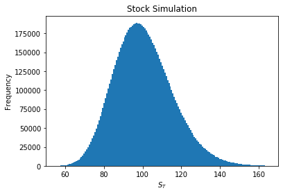
Below we simulate 10 million terminal stock prices, this should be sufficient to get a good approximation of the true distribution of stock prices at expiration.
S=100.0 # spot stock price
K=115.0 # strike
T=0.25 # maturity
r=0.02  # risk free rate
sigma=0.3  # annualized volatility
Ndraws = 10_000_000


np.random.seed(0)
dS = np.random.normal((r - sigma**2/2)*T , sigma*np.sqrt(T), size=Ndraws)
ST = S0 * np.exp(dS)


n, bins, patches = plt.hist(ST,bins=250);
plt.xlabel('$S_T$')
plt.xlim([50,170])
plt.ylabel('Frequency')
plt.title('Stock Simulation')
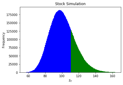
2) Calculate how often The stock is greater than the strike price.
Imagine zipping along the x axis of the histogram above, and adding one to the total if the stock price from the draw is greater than the strike. We then count the number of ones and divide this sum by the number of draws which is 10 million in this case.
The formula for this is shown below where \(1\) is the indicator function returning 1 or 0 dependent upon the condition being satisfied. The formula below represents the probability the stock is above the strike at expiration. Arguably we should we using an integral here as in the previous simulation but hopefully this way is more intuitive.
\(\mathbb{P}(S_T >K) =\frac{1}{N} \displaystyle \sum_{i=1}^N \mathbb{1}_{\{ S_T > K\}} \)
The script below shows that the simulation approximates this probability as 16.5%. This should not be confused with the risk-neutral probability. Although viewing the formula here should give a good intuition as to what exactly a risk-neutral probability actually is when we encounter it later on in the article.
n, bins, patches = plt.hist(ST,bins=250);
plt.xlabel('$S_T$')
plt.xlim([50,170])
plt.ylabel('Frequency')
plt.title('Stock Simulation')
for c, p in zip(bins, patches):
    if c > K:
        plt.setp(p, 'facecolor', 'green')
    else:
        plt.setp(p, 'facecolor', 'blue')


timesInMoney = len(ST[ST>K])

P = timesInMoney/Ndraws
print('The Option was in the money ', f'{timesInMoney} times')
print(f'Out of {Ndraws} simulations')
print(f'Probability of being in the money {P}%')

#The Option was in the money  1651856 times
#Out of 10000000 simulations
#Probability of being in the money 0.1650933%
From the script above we see that the stock will be greater than the strike approximately 16.5% of the time.
3) Calculate Value of Option.
Let \(Q\) be the payoff from the binary option ($5 in our example) The fair price for the binary option is then as follows.
\(\text{Binary Call Value} = \mathbb{P}(S_T>K) \times Qe^{-rT}\\ \\ 0.82=0.165\times 5e^{(-0.02 \times \frac{1}{4})} \)
So the fair price here is approximately $0.82. You can get the risk-neutral probability by multiplying \(\mathbb{P}(S_T>K) \times e^{-rT}\) if you so wish.
The same procedure can be applied to put options by changing \(\mathbb{P}(S_T>K) \times e^{-rT} \ \text{to} \ \mathbb{P}(S_T<K) \times e^{-rT}\) the function below can be used to try different options parameters.
def monte_carlo_binary(S, K, T, r, sigma, Q,
                       type_='call', Ndraws=10_000_000, seed=0):
    np.random.seed(seed)
    dS = np.random.normal((r-sigma**2/2)*T, sigma*np.sqrt(T),size=Ndraws)
    ST = S *np.exp(dS)
    if type_ =='call':
        return len(ST[ST>K])/Ndraws * Q *np.exp(-r*T)
    elif type_ == 'put':
        return len(ST[ST<K])/Ndraws *Q*np.exp(-r*T)
    else:
        raise ValueError('Type must be put or call')


monte_carlo_binary(S, K, T, r, sigma, 5)

#0.8218086669146537
Black-Scholes Closed Form
We can also use the Black-Scholes formula to price binary options, for this we will need the d2 from the previous article. The formulae for calls and puts are given below.
Call formula and Python Implementation
\(Qe^{-rT}N(d_2)\)
from scipy.stats import norm

S=100.0 # spot stock price
K=115.0 # strike
T=0.25 # maturity
r=0.02  # risk free rate
sigma=0.3  # annualized volatility


def d2(S, K, T, r, sigma):
    return (np.log(S/K) + (r- sigma**2 / 2)*T) /  (sigma*np.sqrt(T))

def binary_call(S, K, T, r, sigma, Q=1):
    N = norm.cdf
    return np.exp(-r*T)* N(d2(S,K,T,r,sigma)) *Q
Let's just take a moment to equate some concepts from the Monte-Carlo method we discussed. Notice that when we pass Q=1 in we get a closed form solution to the probability the stock will finish in the money.
\(\mathbb{P}(S_T>K) \times e^{-rT} = N(d1)\)
\(0.165\times e^{(-0.02 \times \frac{1}{4})} = N(d1)\)
binary_call(S, K, T,  r , sigma, Q = 1)
#0.16435024380749158

print(P*np.exp(-r*T)
#0.16436173338293072
Notice that we can recover the probability value we got from the Monte-Carlo simulation by the following.
\(\mathbb{P}(S_T>K) = N(d1)\times e^{rT} \)
\(0.165 = e^{(0.02 \times \frac{1}{4})} N(d1)\)
binary_call(S, K, T,  r , sigma, Q = 1) * np.exp(r*T)

#0.16517405283282427
And Pricing our example option we get approximately the same value. Increasing the Ndraws parameter will reduce this error, however we see below it is fairly accurate and they are in fact measuring the same quantity.
binary_call(S, K, T,  r , sigma, Q =5)
#0.8217512190374578

monte_carlo_binary(S, K, T, r, sigma, 5)
#0.8218086669146537
Put formula and Python Implementation
The formula for pricing a binary put option is given below, in this case we are measuring the probability of the stock being below the strike price.
\(Qe^{-rT}N(-d_2)\)
def binary_put(S, K, T, r, sigma, Q=1):
    N = norm.cdf
    return np.exp(-r*T)* N(-d2(S,K,T,r,sigma)) *Q
Let's try that formula out on pricing a put option with the same parameters as the call we have used throughout this article
binary_put(S, K, T,  r , sigma, Q = 1)
#4.153311176925954

monte_carlo_binary(S, K, T, r, sigma, 5, 'put')
# 4.153253729048758
Now consider if we could have inferred this value without actually using either formula. Since we know that the problem is binary i.e. one of the two events must occur, the stock is either above the strike or below it, the following relationship must hold
\(\mathbb{P}(S_T>K) + \mathbb{P}(S_T<K) = 1\)
To adjust this for a risk neutrality argument we can state the equality shown below. Let \(C_k\ \text{and} \ P_k\) be the prices of digital calls and puts respectively.
\(e^{rT}(C_k + P_k) = 1\)
np.exp(r*T)*(binary_call(S,K,T, r, sigma, Q=1)     +binary_put(S,K,T, r, sigma, Q=1))

#1.0
And then it follows that to price a non-digital binary:
\(e^{rT}(C_K + P_K) = Q\)
Clearly once we know the price of a binary call option we can then infer the price of the put.
\(P_K = e^{-rT}Q -C_K\)
Q = 5
print(np.exp(-r*T)*Q - (binary_call(S,K,T, r, sigma, Q=Q)) )
# 4.153311176925953


print(binary_put(S,K,T, r, sigma, Q=Q))
#4.153311176925954
Summary
The following points are important to remember in order to fully grasp the next section.
1) \(N(d1)\) from the Black-Scholes formula represents the risk neutral probability of the stock being above the strike at expiration.
2) \(N(-d_2)\) is the risk neutral probability of the stock finishing below the strike at expiration.
Implied Probability Distribution from Market Data
In this mini project we will take some of the things we have learned about binary options and apply them to some real market data. It may be useful to read this article on implied volatility if you are unfamiliar with the concept.
The goal of this section is to create a cdf and pdf of the market's expectations regarding the price of Apple stock on the 19th of February.
To follow along you can either download the market data yourself from github here or you can simply download it using Pandas as shown below.
import pandas as pd

df = pd.read_csv('https://raw.githubusercontent.com/codearmo/data/master/implied_dist_article.csv')

print(df.head())

#
#    K        IV       S         T
#0  55  1.017583  131.97  0.207843
#1  60  0.923829  131.97  0.207843
#2  65  0.871095  131.97  0.207843
#3  70  0.802736  131.97  0.207843
#4  75  0.736331  131.97  0.207843
Notes on the data
1) The data was collected from Yahoo Finance prior to the market open on 28th December 2020
2) All of the options expire on the 19th February 2021
3) The Time to expiration variable T was calculated by taking the number of days and dividing by 255.(Could be more accurate admittedly)
4) It is not clear which value Yahoo Finance uses to calculate implied volatility, however, we won't be dealing with market prices and therefore are making some unrealistic assumptions in order to illustrate the concept. Feel free to try it on different data.
5) We will assume the risk free rate is 0.1% per annum taken from here
Interpolate and Extrapolate Implied Volatility
Here we use a polynomial fit with degree 5 to get our new implied volatility values. Since the highest and lowest strike available is 230 and 55 respectively we are going to extrapolate for values between 1 - 55 . While we do suspect that values towards the end of this distribution are highly likely to be much higher in real life, we will use the following model simply for illustrative purposes.
vols = df.IV.values #volatility values
Ks = df.K.values #Strikes

newK = np.arange(1, 270,0.0001) # new higher resolution strikes

poly = np.polyfit(Ks,vols,5) #create implied vol fit
newVols = np.poly1d(poly)(newK) # fit model to new higher resolution strikes

plt.plot(newK, newVols)
plt.title('Implied Volatility Function')
plt.xlabel('$K$')
plt.ylabel('Implied Vol')
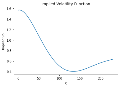
So what we have now is a method to approximate the appropriate volatility values from the data we collected from Yahoo Finance. The reader is encouraged to play around with the function below and compare it with the plot above.
def vol_by_strike(polymdl, K):
    return np.poly1d(polymdl)(K)


vol_by_strike(poly, 131.97)
#0.4038887399619897
So we see from above that the dead on the money volatility is 40.39%
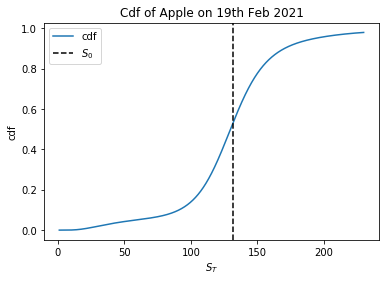
Create Risk Neutral Cumulative Distribution Function for Stock Price at Expiration.
To create a cdf we will want to calculate the weight to the left of the given point, the aforementioned point here is the strike. Referring back to the examples at the beginning of the document we know to calculate this value we can use a digital put option.
S = df.S[0] # extract S_0
T = df['T'][0] #extract T
r= 0.001 # Chosen for convenience

binaries = binary_put(S, newK, T, r, newVols) #calculating the binaries

plt.plot(newK, binaries, label='cdf')
plt.axvline(S,color='black',linestyle='--', label='$S_0$')
plt.xlabel('$S_T$')
plt.ylabel('cdf')
plt.title('Cdf of Apple on 19th Feb 2021')
plt.legend()
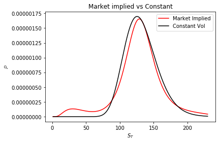
We can then use the following script to assign a probability to each value of \(S_T\) , I hesitate to call this a pdf since we are assigning discrete probabilities to individual price. However, it is useful for illustrative purposes. We will also add a constant volatility distribution i.e. the implied vol at \(S_0\) for comparative purposes.
binaries = binary_put(S, newK, T, r, newVols)

PsT = []  # market implied probabilities

for i in range(1, len(binaries)):

    p = binaries[i] -binaries[i-1]
    PsT.append(p)


constant_vol = vol_by_strike(poly, S)
binaries_const = binary_put(S, newK, T, r, constant_vol)


const_p = []

for i in range(1, len(binaries_const)):

    p = binaries_const[i] -binaries_const[i-1]
    const_p.append(p)


plt.plot(newK[1:], PsT, color='red',label='Market Implied')
plt.plot(newK[1:], const_p, color='black',
         label='Constant Vol')
plt.ylabel('$\mathbb{P}$')
plt.xlabel('$S_T$')
plt.legend()
plt.title('Market implied vs Constant')
Notice that using a constant volatility, there is effectively 0% probability that the stock is below 60 at expiration. However, the market doesn't agree with this idea, perhaps we can interpret this as the risk rare events such as war , natural disaster etc.
Let's explore what we can do with this distribution now that we have it. Let's see how we can calculate the probability that the stock is within a certain interval on the expiration date.
For example say we want to find that risk-neutral probability of :
\(\mathbb{P}(110 < S_T < 140) \)
PsT =np.array(PsT)
idx = np.argwhere((newK[1:] <= 140) & (newK[1:] > 110))
PsT[idx].sum()


# 0.4409622114337626
So according to the market there is a 44.10% chance of the Apple expiring in this interval illustrated below.
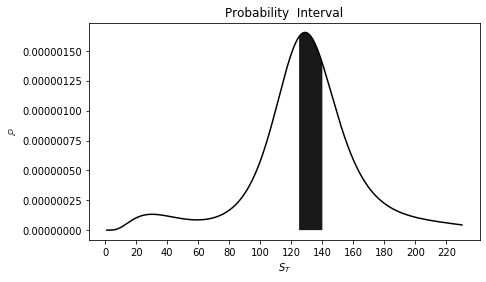
plt.figure(figsize=(7, 4))
plt.plot(newK[1:], PsT, color='black')
plt.fill_between(newK[1:], PsT, where=((newK[1:] < 140)& (newK[1:] > 125)),
                 facecolor='black',alpha=0.9 )
plt.xlabel('$S_T$')
plt.ylabel('$\mathbb{P}$')
plt.title('Probability  Interval')
plt.xticks(np.arange(0,230, 20.0));
Trading Strategy Implications
Recall the strategies illustrated in previous articles here and here. Let's say a trader has his own model for estimating the density of \(S_T\) at expiration, if the model predicts a larger density than the market is implying, the trader could take a long position in a butterfly spread or if the opposite were true he could take a short position in a butterfly.
Hopefully this article has helped you make a connection between probabilities implied by option prices and also an intuitive understanding of risk-neutral probabilities and what they actually mean.