Let's pick up where we left off with the code from part-1. If you are just joining, you can run the script below to download the stock prices for Facebook, Amazon, Apple, Netflix and Google using Pandas datareader.
import pandas_datareader.data as web
import pandas as pd
import datetime as dt
import matplotlib.pyplot as plt
plt.style.use('fivethirtyeight')

start = dt.datetime(2015,1,1)
end = dt.datetime(2020, 1,1)

symbols = ['FB', 'AMZN', 'AAPL',
           'NFLX', 'GOOG']

source = 'yahoo'

data = web.DataReader(symbols, source, start, end)['Adj Close']

data.head()

##converting the data into percentage returns
data  = data.pct_change(periods=1).dropna()
Covariance between two series with Pandas .cov() function
Covariance is a useful statistical measure to describe the joint variability of two series. Putting the formula below into the context of our problem, say for example \(S_a\) is Facebook and \(S_b\) is Amazon or one of the others. \(\mu_a and \ \mu_b\) are the mean daily returns for each stock as explained in part-1.
\(cov\left(S_a,S_b\right)=\frac{1}{N}\sum\limits_{i=1}^{N}\left(S_{a_{i}}-{\ \ \mu}_a\right)\left(S_{b_{i}} -\mu_b\right)\)
Thinking of \(\mu\) as the expected value, we can interpret a positive covariance as: when \(S_a\) is above/below its expected value, \(S_b\)has a tendency to be above/below its mean also. The opposite would be true of a negative covariance, in that if \(S_a\) has a positive return we would expect \(S_b \)to have a negative return.
Let's calculate the covariance between Facebook (FB) and Amazon (AMZN):
data.FB.cov(data.AMZN)
Out[46]: 0.00018649287914951587
Apple (AAPL) and Netflix (NFLX):
data.AAPL.cov(data.NFLX)
Out[61]: 0.0001508603504742106
Since we only have 5 stocks, which translates to 10 possible combinations for calculating the covariance, we could probably type every combination in this scenario with a bit of copy and pasting. However, what if we had 100 stocks? That would mean 4950 combinations, which is going to get boring real quick to type that all out.
Calculating and Plotting Covariance Matrix
Calculating the covariance matrix in Pandas is very easy:
cov = data.cov()
print(cov)
Symbols        FB      AMZN      AAPL      NFLX      GOOG
Symbols
FB       0.000316  0.000186  0.000128  0.000189  0.000161
AMZN     0.000186  0.000340  0.000142  0.000233  0.000179
AAPL     0.000128  0.000142  0.000245  0.000151  0.000123
NFLX     0.000189  0.000233  0.000151  0.000689  0.000185
GOOG     0.000161  0.000179  0.000123  0.000185  0.000229
Let's visualize the covariance matrix using the seaborn library, can you >>>pip install seaborn if you don't have it yet.
import seaborn as sns
import numpy as np

fig, ax = plt.subplots(figsize=(10, 8))

sns.heatmap(corr,vmin=-0.0002,
            cmap=sns.color_palette("Reds",100),
            square=True, ax=ax, annot=True)
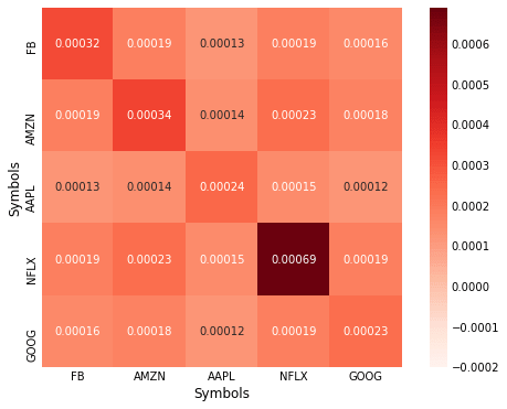
Since all our variables are on the same scale, it is easy to compare and contrast the relationship between them. However, often when analyzing other variables this won't be the case and comparing covariances will become difficult.
Correlation Matrix with Pandas
Correlation can be thought of as a normalized version of covariance. To get an intuitive understanding of how to interpret the correlation coefficient, consider taking the covariance of a series with itself, this results the variance, take the square root of each number on the diagonal of the covariance matrix above, and notice how it is the same as the standard deviation from part-1. Compare the two formulas and you can see why this is so.
Formula for Pearson's correlation:
\(\rho = \frac{cov(S_a,S_b)}{\sigma_a \sigma_b}\)
Think again of taking the covariance of a series with itself and plugging it into the formula above \(\rho = \frac{cov(S_a,S_a)}{\sigma_a^2 } = \frac{\sigma^2}{\sigma^2}= 1\) , if we were to take the correlation of a variable with the negative of itself we would get -1.0 as a move upwards in one series gets an equal move in the opposite direction. The correlation coefficient therefore returns a value between 1.0 and -1.0.
The syntax for calculating the correlation coefficient in Pandas is similar to the way we calculated covariance.
data.FB.corr(data.AMZN)
Out[79]: 0.5693718048486351
Calculating the correlation matrix:
corr = data.corr(method='pearson')

print(corr)
Out[80]:
Symbols        FB      AMZN      AAPL      NFLX      GOOG
Symbols
FB       1.000000  0.569372  0.460122  0.405471  0.599375
AMZN     0.569372  1.000000  0.492522  0.482430  0.640953
AAPL     0.460122  0.492522  1.000000  0.367275  0.521428
NFLX     0.405471  0.482430  0.367275  1.000000  0.466755
GOOG     0.599375  0.640953  0.521428  0.466755  1.000000
Plotting the correlation matrix:
fig, ax = plt.subplots(figsize=(8, 6))

sns.heatmap(corr,vmin=0,vmax=1,
            cmap=sns.color_palette("Reds",100),
            square=True, ax=ax, annot=True)
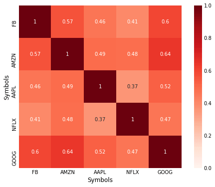
Nice plot for such little work! You can see the seaborn docs for information on configuring the options to change the appearance of the heatmap.
Spearman's Rank Correlation
Spearman's rank correlation is most useful for data that is ordinal in nature. However, it is also useful if the data contains outliers, look back to the covariance formula and consider a large one-off deviation, and the effect this is likely to have on the correlation coefficient.
See Wikipedia entry which has a useful example regarding IQ and hours of television watched per week.
In Pandas we just have to change the method to 'spearman':
data.corr(method='spearman')
Out[92]:
Symbols        FB      AMZN      AAPL      NFLX      GOOG
Symbols
FB       1.000000  0.597812  0.468402  0.454571  0.649423
AMZN     0.597812  1.000000  0.499789  0.498702  0.673243
AAPL     0.468402  0.499789  1.000000  0.373772  0.530188
NFLX     0.454571  0.498702  0.373772  1.000000  0.468844
GOOG     0.649423  0.673243  0.530188  0.468844  1.000000
Read Next Article