In order to show some basic statistics with Pandas, we will be using a real life data-set in this article, as it is often easier to show the concepts when applied in context. Since financial data is so readily available from Yahoo Finance, let's use some stock data to demonstrate calculating statistics with Pandas. Where possible a brief explanation of the stats will be given for those unfamilar with the methods. The stocks we will be using for this article are known as the FAANG stocks, which consists of Facebook, Amazon, Apple , Netflix and Google.
Pandas functions covered:
- mean
- pct_change
- standard deviation
- mean absolute deviation
- skew
Import the necessary libraries and download the FAANG data for 2015-2020
import pandas_datareader.data as web
import pandas as pd
import datetime as dt
import matplotlib.pyplot as plt
plt.style.use('fivethirtyeight')


start = dt.datetime(2015,1,1)
end = dt.datetime(2020, 1,1)

##ticker symbols for FAANG stocks
symbols = ['FB', 'AMZN', 'AAPL',
           'NFLX', 'GOOG']

source = 'yahoo'

## take only adjusted close prices
data = web.DataReader(symbols, source, start, end)['Adj Close']

data.head()
Out[226]:
Symbols            FB        AMZN        AAPL       NFLX        GOOG
Date
2015-01-02  78.449997  308.519989  100.216454  49.848572  523.373108
2015-01-05  77.190002  302.190002   97.393181  47.311428  512.463013
2015-01-06  76.150002  295.290009   97.402374  46.501427  500.585632
2015-01-07  76.150002  298.420013   98.768150  46.742859  499.727997
2015-01-08  78.180000  300.459991  102.563072  47.779999  501.303680
That looks as expected.
I will use the population measures, which isn't strictly correct, however, the difference is likely negligible for the purposes of this article.
Mean
Let's calculate the arithmetic mean \(\mu\) for each stock:
\(\mu=\ \frac{1}{N}\sum\limits_{i=1}^{N }x_i\)
data.mean()
Out[229]:
Symbols
FB       143.073386
AMZN    1115.047337
AAPL     149.094641
NFLX     201.427671
GOOG     913.613379
dtype: float64
For our specific problem, calculating the mean with the raw prices probably doesn't make much sense. Let's check out Pandas pct_change function, to normalize the data as follows:
\(pct\_change\ =\ \frac{Price\ Today\ -\ Price\ t\ periods\ ago}{Price\ Today}\)
The default t in the formula above is 1, however you can override this to any period you wish. Note, that you will always have t NaN values when using this function, therefore we add dropna() to the function to clean the data up.
data = data.pct_change(periods=1).dropna()

data.head()
Out[236]:
Symbols           FB      AMZN      AAPL      NFLX      GOOG
Date
2015-01-05 -0.016061 -0.020517 -0.028172 -0.050897 -0.020846
2015-01-06 -0.013473 -0.022833  0.000094 -0.017121 -0.023177
2015-01-07  0.000000  0.010600  0.014022  0.005192 -0.001713
2015-01-08  0.026658  0.006836  0.038423  0.022188  0.003153
2015-01-09 -0.005628 -0.011749  0.001072 -0.015458 -0.012951
Let's make a bar chart to compare the stocks average daily change
data.mean().plot.bar()
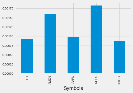
It looks like Netflix has had the highest mean percentage return historically.
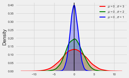
Standard Deviation
The standard deviation is the most commonly used measure of dispersion around the mean. Consider the graph below constructed with mock data for illustrative purposes, in which all three distributions have exactly the same mean (zero). Clearly the red and green curves exhibit more dispersion around the mean, which is due to higher standard deviations.
\(\sigma =\sqrt{\frac{1}{N} \sum\limits_{i=1}^N(x_i-\mu)^2}\)
It may be useful to mention that the standard deviation is only used to describe continuous data, if you had categorical or nominal data, it wouldn't make sense to use standard deviation to describe your data. For our particular problem, standard deviation is a widely used measure of the riskiness of a stock, see this Investopedia article for more information.
Let's calculate the daily standard deviation for each of our FAANG stocks and compare them in a bar chart.
data.std().plot.bar()
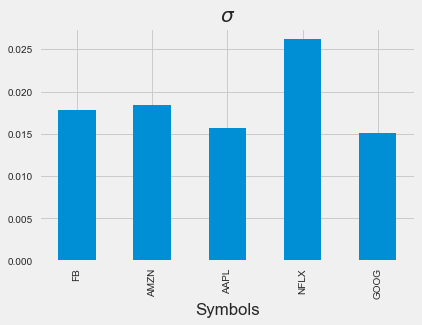
Looks like Netflix has the highest standard deviation of the stocks in our sample.
Mean Absolute Deviation (MAD)
The formula below is much more intuitive, and arguably a better measure for dispersion. See this interesting discussion on stackexchagne regarding the differences between standard deviation and MAD
\(\frac{1}{N} \sum\limits_{i=1}^N |x_i-\mu|\)
data.mad()
Out[303]:
Symbols
FB      0.011882
AMZN    0.012194
AAPL    0.011016
NFLX    0.017820
GOOG    0.010189
dtype: float64
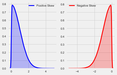
Skew
Skew, also known as the third moment of the distribution, is a measure of assymetry in the distribution. Notice, the cubed term in the formula below, which allows for both negative and positive values. The plot below with mock data contrasts distributions with positive and negative skew. Negatively skewed distributions have heavier tails, meaning they have more extreme negative values, with the opposite being true for positively skewed distributions.
\(Skew = {\frac{1}{N}}\ \sum\limits_{i=1}^N \frac{(x_i-\mu)^3}{\sigma^3}\)
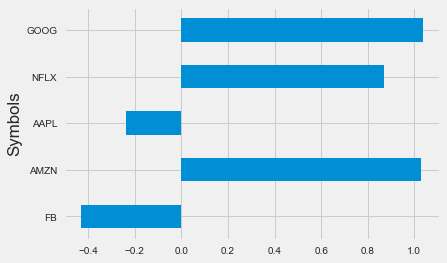
Let's compare the skewness measure for the stocks in our sample:
data.skew().plot.barh()
Full script for this article
import pandas_datareader.data as web
import pandas as pd
import datetime as dt
import matplotlib.pyplot as plt
plt.style.use('fivethirtyeight')

start = dt.datetime(2015,1,1)
end = dt.datetime(2020, 1,1)

symbols = ['FB', 'AMZN', 'AAPL',
           'NFLX', 'GOOG']

source = 'yahoo'

data = web.DataReader(symbols, source, start, end)['Adj Close']

data.head()

data  = data.pct_change(periods=1).dropna()

data.mean().plot.bar()

data.std().plot.bar()

data.mad()


data.skew().plot.barh()