Are you looking to take your cryptocurrency trading to the next level? Look no further than Bybit, the leading crypto derivatives exchange. With advanced trading tools, low fees, and a user-friendly platform, Bybit makes it easy to trade Bitcoin, Ethereum, and other popular cryptocurrencies. And if you sign up using our affiliate link through Codearmo and use the referral code CODEARMO, you'll receive exclusive benefits and bonuses up to $30,000 to help you get started. Don't miss out on this opportunity to join one of the fastest-growing communities in crypto trading. Sign up for Bybit today and start trading like a pro!
Contents
- Description of Markowitz Portfolio Optimization
- Data Collection
- Minimum Variance
- Maximum Short
- Introducing Short Sales
- Comparison of Bybit Spot balances to Optimal Weights
What is Markowitz Portfolio Optimization?
Markowitz portfolio optimization is a mathematical framework that helps investors to maximize their expected return for a given level of risk. The basic idea behind this theory is that by diversifying a portfolio across multiple assets, investors can reduce the overall risk while still achieving a desired level of return.
In practice, Markowitz portfolio optimization involves calculating the expected return and risk of each individual asset in a portfolio, as well as the correlation between the assets. The optimal portfolio is then constructed by selecting a combination of assets that provide the highest expected return for a given level of risk.
This approach takes into account the fact that different assets have different levels of risk and return, and that the relationship between assets can impact the overall risk and return of a portfolio. The goal is to create a portfolio that balances risk and return to achieve the best possible outcome for the investor.
While Markowitz portfolio optimization is a powerful tool for portfolio management, it is not without limitations. Some of the challenges include the need for accurate inputs (such as expected returns and correlations), the assumption of a normal distribution of returns, and the fact that historical performance may not be a reliable predictor of future performance. Additionally, the optimization process can be computationally intensive, particularly when dealing with large portfolios.
Terminology & Notation
For readers interested in the underlying mathematics behind portofolio optimization, however, the University of Washington has a very nice guide which can be found here. We will not be deriving, or going in to any depth regarding the math, however, we will provide some hands-on python examples.
\(x = \) vector of weights , i.e. \(x_i\) where the ith element is Bitcoin \(x_i\) = 0.40 , would represent a 40% allocation in Bitcoin.
\(\Sigma =\) covariance matrix of an crypto returns.
\(\mu = \) vector of average returns for each crypto asset, i.e. \(\mu_i\) where the ith element is Bitcoin \(\mu_i\) = 0.002 , would represent a 0.2% average return return for Bitcoin.
The return of a portfolio will then be \(x^Tu\) = weights x average returns.
The variance of a portfolio will then be \(x^T\Sigma x\) which represents a weighted sum of the variance of each asset along with the weighted covariance of each asset with all other assets. Better to see guide listed above for more info and some nice examples.
Data Collection
In order to avoid clutter, 3 functions related to data collection (get_last_timestamp, format_data, get_all_data) can be found at the end of this article, if you want to follow along please copy and paste them in prior to running the code below.
In this article, we will be discussing a universe of 10 of the largest cap coins, as of the time of writing. To retrieve data for our analysis, you won't need an API key, but if you're interested in setting one up, we recommend checking out this article. If you do decide to use an API key, make sure to remove the key logic from the HTTP object below, as indicated in the comments.
For our analysis, we will be using daily data. Running the code snippet below will provide us with a dataframe containing the close prices for each of the assets in the symbols list. Of course, you can experiment with different intervals and larger numbers of symbols, depending on your specific needs.
from pybit.unified_trading import HTTP
from scipy.optimize import minimize
import matplotlib.pyplot as plt
import datetime as dt
import json
import time
import pandas as pd


with open('authcreds.json') as j:
        creds = json.load(j)


key = creds['KEY_NAME']['key']
secret = creds['KEY_NAME']['secret']

session = HTTP(api_key=key, api_secret=secret, testnet=False)

#if you live in a prohibited area you can follow along by removing keys, although you
#won't be able to follow along with account specific parts of this article.
session = HTTP(testnet=False)

interval = 'D'

symbols = ['BTCUSDT', 'ETHUSDT', 'BNBUSDT',
           'XRPUSDT', 'ADAUSDT', 'DOGEUSDT',
           'MATICUSDT', 'SOLUSDT', 'DOTUSDT',
               'LTCUSDT']

dfs = []

for symbol in symbols:
    data = get_all_data(symbol, interval)
    dfs.append(data)

df = pd.DataFrame(data=dfs[0].close)


for data in dfs[1:]:
    df = pd.merge(df, pd.DataFrame(data.close), left_index=True, right_index=True)


df.columns = symbols
df =df[~df.index.duplicated(keep='last')]

'''
            BTCUSDT  ETHUSDT  BNBUSDT  ...  SOLUSDT  DOTUSDT  LTCUSDT
timestamp                              ...
2021-06-29  35918.5  2165.05   300.95  ...   33.960   16.290   144.19
2021-06-30  35018.0  2273.25   302.80  ...   35.485   16.360   144.09
2021-07-01  33490.0  2107.00   287.65  ...   33.300   15.170   137.23
2021-07-02  33753.5  2152.75   287.15  ...   33.975   15.290   136.80
2021-07-03  34649.5  2226.55   298.20  ...   34.510   15.515   140.07

[5 rows x 10 columns]
'''
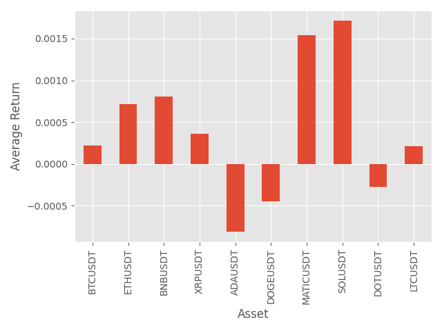
Calculate and visualize vector of mean returns, note this is \(\mu\) from the terminology section at the beginning of this article
mean_rets = df.pct_change().mean().values.T
df.pct_change().mean().plot.bar()
plt.xlabel('Asset')
plt.ylabel('Average Return')
plt.tight_layout()
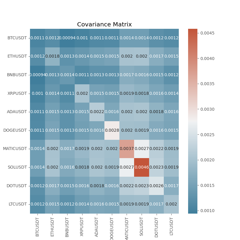
Create the covariance matrix
cov_mat = df.pct_change().cov()

f, ax = plt.subplots(figsize=(8,8))
cmap = sns.diverging_palette(230, 20, as_cmap=True)
sns.heatmap(cov_mat, annot=True, cmap=cmap)
plt.title('Covariance Matrix')
Minimum Variance Portfolio
The minimum variance portfolio is the set of weights that provide the lowest possible variance as the name suggests. We will be using scipy's sequential least squares method to solve this problem.
Recall that the variance for a portfolio is \(x^T\Sigma x\) therefore we want to solve for the weights \(x\) vector such that this \(x^T\Sigma x\) quantity is minimized. We will add some addition constraints the first of which is that the elements of \(x\) must sum to 1 meaning we are fully invested, in addition we will constrain the problem such that the weights are non-negative, therefore our optimization problem takes the form:
\(\underset{x}{\text{min} } \; \;{ x^T\Sigma x} \; \)
subject to
\(x^T1 = 1 ,\)
\(x_i >= 0 , \text{for all} \;i=1,.....n \)
where \(n=\)number of assets
You will also notice a list of tuples, these relate to the bounds, where we can define the non negative constraint.
def min_var_obj(x):
    '''
    { x^T\Sigma x}
    '''

    return x.T@cov_mat@x

def sum_to_one_cons(x):
    '''
    constraint
    x^T1 = 1
    '''
    return np.sum(x) - 1


cons =({'type':'eq', 'fun': sum_to_one_cons},)

# here we constrain possible solutions, meaning theynon-negative
bounds = [(0,1) for _ in range(len(mean_rets))]

#this is intitial guess for optimizer, note this is same as equal weihgs
# previosuly discussed
x0 = np.repeat(1/len(symbols), len(symbols))

res = minimize(obj,x0=equal_w,
               method='SLSQP',
               bounds=bounds,
               constraints=cons)

for sym,weight in zip(symbols, res.x):
    print(f'Weight for {sym} is {weight.round(4)}')

'''
Weight for BTCUSDT is 0.7721
Weight for ETHUSDT is 0.0
Weight for BNBUSDT is 0.2279
Weight for XRPUSDT is 0.0
Weight for ADAUSDT is 0.0
Weight for DOGEUSDT is 0.0
Weight for MATICUSDT is 0.0
Weight for SOLUSDT is 0.0
Weight for DOTUSDT is 0.0
Weight for LTCUSDT is 0.0
'''
As we can see from above, this allocation strategy, only assigns weights to 2 assets BTC & BNB , this is probably not what we want, since by selecting the universe we did, sort of implicitly means we want to have some position in each asset. If we wanted to do this we could define a minimum or maximum weight, let's try saying we must have strictly positive weights, along with a max position of 20% per asset.
bounds = [(0.001,0.2) for _ in range(len(mean_rets))]
res = minimize(obj,x0=equal_w,
               method='SLSQP',
               bounds=bounds,
               constraints=cons)


for sym,weight in zip(symbols, res.x):
    print(f'Weight for {sym} is {weight.round(4)}')

'''
Weight for BTCUSDT is 0.2
Weight for ETHUSDT is 0.1988
Weight for BNBUSDT is 0.2
Weight for XRPUSDT is 0.2
Weight for ADAUSDT is 0.0694
Weight for DOGEUSDT is 0.0176
Weight for MATICUSDT is 0.001
Weight for SOLUSDT is 0.001
Weight for DOTUSDT is 0.001
Weight for LTCUSDT is 0.1112
'''
Add a Target Return
The following section will give some nice intuition about the concept behind portfolio optimization, we are going to add an equality constraints such that the optimizer will select the weights of the portfolio such that \(x^T\mu= target\) , note the code below is the same stuff we did above, only in a function with another equality constraint.
def optimize_min_var_portfolio(mean_rets, cov_mat, bounds, target_ret, cons):

    if target_ret:

        target_eq = lambda x: x.T @ mean_rets - target_ret
        cons += ({'type': 'eq', 'fun': target_eq},)

    #perform minimization

    x0 = np.repeat(1/len(mean_rets), len(mean_rets))

    def obj(x):
        return x.T@cov_mat@x


    res = minimize(fun=obj, x0=x0, method='SLSQP',
                   bounds=bounds, constraints=cons,
                   tol=1e-8)
    return res.x, res.fun


target_rets = np.arange(mean_rets.min(), mean_rets.max(), 0.00001)

port_rets = np.zeros_like(target_rets)
port_sigma = np.zeros_like(target_rets)

bounds = [(0,1) for _ in range(len(mean_rets))]
cons =({'type':'eq', 'fun': sum_to_one_cons},)
for idx, target in enumerate(target_rets):
    weights, sigma = optimize_min_var_portfolio(mean_rets, cov_mat, bounds, target, cons)
    port_ret = weights.T@mean_rets
    port_rets[idx] = port_ret
    port_sigma[idx] = np.sqrt(weights.T@cov_mat@weights)


fig, ax = plt.subplots()
ax.scatter(port_sigma, port_rets, s=3,color='black')

asset_vars = np.sqrt(np.diag(cov_mat))

for i, symbol in enumerate(symbols):
    ax.scatter(asset_vars[i], mean_rets[i], marker='o')
    ax.annotate(symbol,(asset_vars[i], mean_rets[i]) )
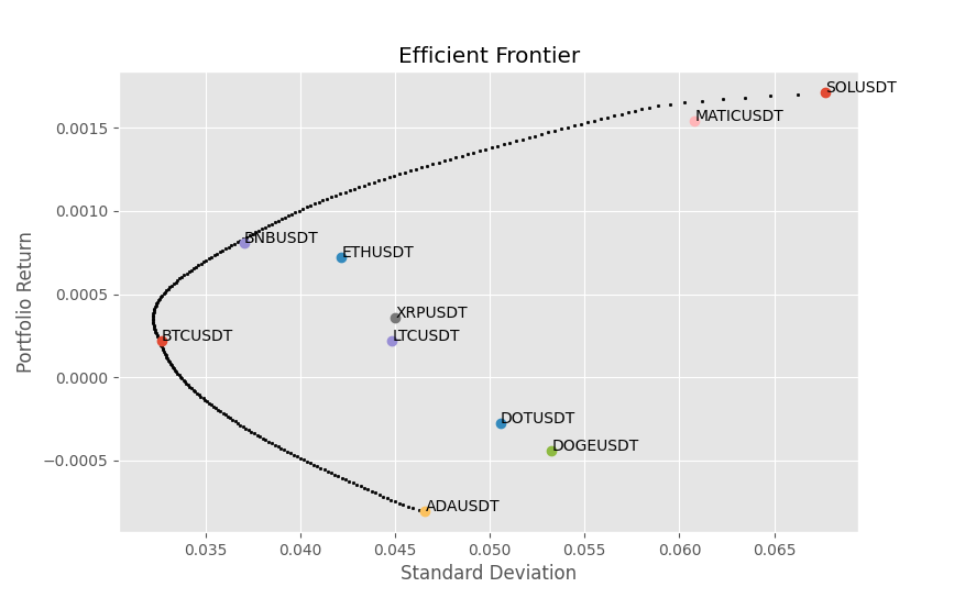
Although this is not a perfect example,lets take ETH for instance, if these measurements of standard deviation and average return are accurate, then it would not be ratioanal to put 100% in ETH , since there is a portfolio above it that offers a high return for the same level of risk. This is the whole idea behind the Markowitz optimization, we want the optimal set of assets for a given target return, and an increase in the level of risk defined as the standard deviation must come with an increase in return. A way to think of this visually is, take any point within the feasible set of solutions, if there exists a black dot in a vertical direction above it, then there exists a portflio that has a higher return for the same level of risk.
Maximum Sharpe Ratio Optimization
The Sharpe ratio is a measure of the risk-adjusted return of an investment or portfolio. It was developed by Nobel laureate William F. Sharpe in 1966. The ratio is calculated by subtracting the risk-free rate of return from the expected return of the investment, and then dividing by the standard deviation of the investment's return.
Sharpe Ratio = Expected Return / Standard Deviation
The Sharpe ratio is useful because it provides a way to compare the returns of different investments while taking into account the level of risk involved. A higher Sharpe ratio indicates that an investment has provided higher returns relative to the risk taken.
So the problem definition is quite similar to the minimum variance problem.
\(\underset{x}{\text{max} } \; \; {\frac{x^T\mu}{\sqrt{ x^T\Sigma x}}} \; \)
subject to
\(x^T1 = 1 ,\)
\(x_i >= 0 , \text{for all} \;i=1,.....n \)
where \(n=\)number of assets
Note here that we need to add the minus sign so that the minimization problem becomes a maximization one.
def max_sharpe_obj(x):
    return -(mean_rets @ x) / (np.sqrt(x.T@cov_mat@x))


cons =( {'type':'eq', 'fun': sum_to_one_cons},
       )
bounds = [(0,1) for _ in range(len(symbols))]
res = minimize(fun=max_sharpe_obj,x0=x0, bounds=bounds, method='SLSQP',constraints=cons)

print(list(zip(symbols, res.x)))
'''
[('BTCUSDT', 0.0), ('ETHUSDT', 0.0), ('BNBUSDT', 0.20386416844096306), ('XRPUSDT', 0.0), ('ADAUSDT', 5.612428753243661e-20), ('DOGEUSDT', 1.493033446276062e-18), ('MATICUSDT', 0.38129426896063395), ('SOLUSDT', 0.41484156259840316), ('DOTUSDT', 2.0865308856359004e-17), ('LTCUSDT', 0.0)]
'''
So we see that for the max sharpe portfolio, the allocations are nearly all to BNB, SOL & MATIC, we will discuss in the limitations part about why this might be.
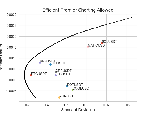
Allowing Short Sales
Sometimes, an investor may take the view that an asset is going to underperform, and therefore wants to take a position such that he will profit in the event of the asset losing value. Lets say we are allowed to take short positions, we need to be careful here, as the minimization procedure will happily come up with strange values if it is not constrained correctly, so we will take an example of an investor who is not allowed to take more than 100% of total equity exposure, so that means the absolute value of the weights must sum to 1. We could of course, just do it such that all the weights still sum to 1 allowing more than 1x gross exposure, we would simply use the previous constraint.
We will also add that the investor has decided that a single short position , must be at most 10% of equity.
GROSSEXP = 1
def gross_exposure_const(x):
    '''
    constraint
    x^T1 = 1
    '''
    return np.abs(np.sum(x)) - GROSSEXP


cons =( {'type':'eq', 'fun': gross_exposure_const},
       )


bounds = [(-0.1,1) for _ in range(len(symbols))]
w, sigma = optimize_min_var_portfolio(mean_rets, cov_mat, bounds, 0.001, cons)

target_rets = np.arange(mean_rets.min(), mean_rets.max()*2, 0.00001)

port_rets = np.zeros_like(target_rets)
port_sigma = np.zeros_like(target_rets)

cons =({'type':'eq', 'fun': gross_exposure_const},)
for idx, target in enumerate(target_rets):
    weights, sigma = optimize_min_var_portfolio(mean_rets, cov_mat, bounds, target, cons)
    port_ret = weights.T@mean_rets
    port_rets[idx] = port_ret
    port_sigma[idx] = np.sqrt(weights.T@cov_mat@weights)


fig, ax = plt.subplots()
ax.scatter(port_sigma, port_rets, s=3,color='black')

asset_vars = np.sqrt(np.diag(cov_mat))

for i, symbol in enumerate(symbols):
    ax.scatter(asset_vars[i], mean_rets[i], marker='o')
    ax.annotate(symbol,(asset_vars[i], mean_rets[i]) )

plt.title('Efficient Frontier Shorting Allowed')
plt.ylabel('Portfolio Return')
plt.xlabel('Standard Deviation')
Limitations
The most natural question is whether this sort of optimization is at all useful in the context of a portfolio of crypto assets. Below we list some general and idiosyncratic drawbacks and limitations to optimization procedure.
- Our sample is very small and encompasses what was a prolonged bear market, this undoubtedly skews the results.
Potential Fix: Get a larger dataset that includes different market regimes.
- The Sharpe ratio assumes that the returns are normally distributed, i.e. 0 skew, we know that in crypto assets can have extremely large downside moves. Lets take Solana for instance, which the optimization has allocated a rather large weight to in many of the iterations from above.
Potential Fix: Maybe you could try to minimze the Sortino ratio, which replaces the variance in with the semi-variance i.e. only downside moves are considered, and then optimize on this.
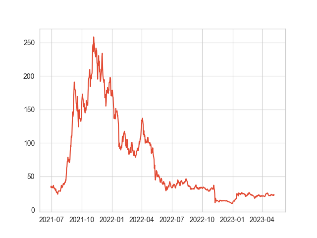
- Using point estimates for mean and covariances, is probably not a good idea, lets take SOLUSDT for example, as can be seen from the mean returns we have used in the models above, SOL has the highest expected daily return, however, when we look at the plot for SOL it would have been a bit of a disaster if we had used this as the input to an optimization model, as it would have massively over weighted SOL leading to us getting badly wrecked in 2022.
'''
{'BTCUSDT': 0.00021933003625132586,
 'ETHUSDT': 0.0007188773032525807,
 'BNBUSDT': 0.0008050841099479799,
 'XRPUSDT': 0.0003610798044561819,
 'ADAUSDT': -0.0008073168797176055,
 'DOGEUSDT': -0.0004438213220123372,
 'MATICUSDT': 0.001539259949180541,
 'SOLUSDT': 0.0017118822216878056,
 'DOTUSDT': -0.00027470229689660706,
 'LTCUSDT': 0.00021683360542821197}

'''

plt.plot(df.SOLUSDT)
Potential Fix: Well we can recognize that returns are very difficult to predict accurately, therefore we might want to use some fundamental prediction, in context of stock market, maybe analyst predictions would be useful to put in here. Therefore, you might try to come up with some consensus prediction regarding expected returns and insert that in to the model.
expected_returns = {'BTCUSDT': 'insert_prediction',
                     'ETHUSDT': 'insert_prediction',
                     'BNBUSDT': 'insert_prediction',
                     'XRPUSDT': 'insert_prediction',
                     'ADAUSDT': 'insert_prediction',
                     'DOGEUSDT': 'insert_prediction',
                     'MATICUSDT': 'insert_prediction',
                     'SOLUSDT': 'insert_prediction',
                     'DOTUSDT': 'insert_prediction',
                    'LTCUSDT': 'insert_prediction'}
In addition, perhaps it is more an art than a science in choosing the bounds, therefore we could use some sort of market cap rule or something similar. Or maybe some sort of volatility/ correlation forecasting would be useful.
bounds = [(insert lowerBTC, insert higher BTC), (), ....., ]
Another possible way to estimate the means of the asset is to take the daily return such that it is fit to the data we have the compounded mean return.
Take the following:
\(A_t = \text{Asset price at time t} \; , \: t \: \text{in} \; {0, 1, ...., T}\)
\(u_i = (\frac{A_T}{A_0})^{ \frac{1}{T}} -1\)
So lets compare the mean returns using the compounded mean return.
mean_rets = df.pct_change().mean().values.T

realized_means = ((df[:1].values / df[-1:].values)**(1/len(df)) -1 ).T


for i in range(len(symbols)):
    print(f'{symbols[i]} , avg_ret = {mean_rets[i]}, comp = {realized_means[i]}')


'''
BTCUSDT , avg_ret = 0.00014245801265624404, comp = [0.0003907]
ETHUSDT , avg_ret = 0.000643981110890745, comp = [0.00024378]
BNBUSDT , avg_ret = 0.0007386822695431426, comp = [-4.93423454e-05]
XRPUSDT , avg_ret = 0.00025607663289021327, comp = [0.00073881]
ADAUSDT , avg_ret = -0.0008696773466177692, comp = [0.001945]
DOGEUSDT , avg_ret = -0.0005295588579693877, comp = [0.00189407]
MATICUSDT , avg_ret = 0.0013479034615124844, comp = [0.00044712]
SOLUSDT , avg_ret = 0.0015781816184812065, comp = [0.00072983]
DOTUSDT , avg_ret = -0.0003337828202600325, comp = [0.00160919]
LTCUSDT , avg_ret = 0.00015536051549678545, comp = [0.00085429]
'''
So we see the numbers are quite different. If you know of some reason why this approach should not be used get in contact here with reason.
Optimizing Your Bybit Portfolio
For this section, you will need to have created an API key and have some non-zero balances of assets. We will be optimizing a portfolio of USDT futures, you can of course change this to SPOT category , or perhaps you can play around with the script to combine bot spot and futures in to a single portfolio.
Note the script below should serve as a template, hopefully after reading the previous parts of this article you should be able to combine the methods to suit your objectives.
The scripy below will:
- Pull your current positions, category being a member of ['linear' , 'spot', 'inverse'] , the setteCoin parameter should be for example USDT.
- Format and display them in a dictionary form, we get the weights by taking each position value in relation to the total dollar position value as can be seen in the get_current_position_weights function.
- Pull the data for the symbols you have in your portfolio. If you are considering adding new symbols, you would add the symbols to this list e.g. symbols.extend([new, new, new])
- Calculate the minimum variance portfolio weights and print them for the reader to compare to the current weights.
def get_current_positions(category, settleCoin):
    response = session.get_positions(category=category,
                                     settleCoin=settleCoin).get('result')

    pos_list = response.get('list')
    if len(pos_list) == 0:
        print(f'You current have no positions for this category = {category}')
        return

    positions ={}

    for pos in pos_list:
        symbol = pos.get('symbol')
        dollar_value = float(pos.get('markPrice')) * float(pos.get('size'))
        positions.update({symbol: dollar_value})

    return positions


def get_current_position_weights(positions):
    total_dollar_value = sum(positions.values)
    weights = {sym: val/total_dollar_value for sym, val in positions.items()}
    return weights


def display_weights(weights):
    print('Current Weights')
    for sym, w in weights.items():
        print(f'{sym} weight is {round(w,4)}')


positions = get_current_positions(category='linear', settleCoin='USDT')

weights = get_current_position_weights(positions)

display_weights(weights)

symbols = list(weights.keys())

interval = '1D'

dfs = []

for symbol in symbols:
    data = get_all_data(symbol, interval)
    dfs.append(data)

df = pd.DataFrame(data=dfs[0].close)


for data in dfs[1:]:
    df = pd.merge(df, pd.DataFrame(data.close), left_index=True, right_index=True)


df.columns = symbols
df =df[~df.index.duplicated(keep='last')]

mean_rets = df.pct_change().mean().values.T
cov_mat = df.pct_change().cov()


def optimize_min_var_portfolio(mean_rets, cov_mat, bounds, target_ret, cons):

    if target_ret:

        target_eq = lambda x: x.T @ mean_rets - target_ret
        cons += ({'type': 'eq', 'fun': target_eq},)

    #perform minimization

    x0 = np.repeat(1/len(mean_rets), len(mean_rets))

    def obj(x):
        return x.T@cov_mat@x


    res = minimize(fun=obj, x0=x0, method='SLSQP',
                   bounds=bounds, constraints=cons,
                   tol=1e-8)
    return res.x, res.fun

def min_var_obj(x):
    '''
    { x^T\Sigma x}
    '''

    return x.T@cov_mat@x

def sum_to_one_cons(x):
    '''
    constraint
    x^T1 = 1
    '''
    return np.sum(x) - 1


cons =({'type':'eq', 'fun': sum_to_one_cons},)

# here we constrain possible solutions, meaning theynon-negative
bounds = [(0,1) for _ in range(len(mean_rets))]

#this is intitial guess for optimizer, note this is same as equal weihgs
# previosuly discussed
x0 = np.repeat(1/len(symbols), len(symbols))

#you can change the bounds here, note they must be in the same order as the symbols appear
bounds = [(0,1) for _ in range(len(mean_rets))]

w, sigma = optimize_min_var_portfolio(mean_rets, cov_mat, bounds, cons)

print(dict(zip(symbols, weights))
Data Collection Scripts
def format_data(response):
    '''


    Parameters
    ----------
    respone : dict
        response from calling get_klines() method from pybit.
    freq : str
        DESCRIPTION.
        interval that has been passed in to get_klines method, used in order
        to round the datetimes, which will be mapped to pandas freq str

    Returns
    -------
    dataframe of ohlc data with date as index

    '''
    data = response.get('list', None)

    if not data:
        return

    data = pd.DataFrame(data,
                        columns =[
                            'timestamp',
                            'open',
                            'high',
                            'low',
                            'close',
                            'volume',
                            'turnover'
                            ],
                        )

    f = lambda x: dt.datetime.utcfromtimestamp(int(x)/1000)
    data.index = data.timestamp.apply(f)
    return data[::-1].apply(pd.to_numeric)

def get_last_timestamp(df):
    return int(df.timestamp[-1:].values[0])


def get_all_data(sym, interval):

    start = int(dt.datetime(2020, 1, 1).timestamp()* 1000)
    df = pd.DataFrame()
    while True:
        response = session.get_kline(category='linear',
                                     symbol=sym,
                                     start=start,
                                     interval=interval).get('result')

        latest = format_data(response)

        if not isinstance(latest, pd.DataFrame):
            break

        start = get_last_timestamp(latest)

        time.sleep(0.1)

        df = pd.concat([df, latest])
        print(f'Collecting data starting {dt.datetime.fromtimestamp(start/1000)}')
        if len(latest) == 1: break
    return df