Are you looking to take your cryptocurrency trading to the next level? Look no further than Bybit, the leading crypto derivatives exchange. With advanced trading tools, low fees, and a user-friendly platform, Bybit makes it easy to trade Bitcoin, Ethereum, and other popular cryptocurrencies. And if you sign up using our affiliate link through Codearmo and use the referral code CODEARMO, you'll receive exclusive benefits and bonuses up to $30,000 to help you get started. Don't miss out on this opportunity to join one of the fastest-growing communities in crypto trading. Sign up for Bybit today and start trading like a pro!
What are Long-Short Strategies?
A long-short strategy is a popular investment strategy that involves simultaneously buying (going long) some assets and selling (going short) others in order to profit from the relative performance of the two assets. The idea is to identify two assets that are positively correlated (i.e., tend to move in the same direction), but where one is expected to outperform the other. By going long on the expected outperformer and short on the expected underperformer, investors can potentially profit from the difference in performance between the two assets, while reducing their exposure to overall market risk. Long-short strategies are commonly used in equity markets, where they can be implemented using a variety of techniques, such as factor models, statistical arbitrage, and fundamental analysis. They can also be applied to other asset classes, such as commodities, currencies, and cryptocurrencies, using similar principles.
In this article, we will discuss a method for determining the optimal long-short ratio, which involves simultaneously taking long and short positions in two assets. We will introduce the concept of beta, which provides a measure of the relative volatility of an asset compared to a benchmark (such as a market index or another asset), and explain how it can be used to construct a long-short portfolio that balances the risks and returns of the two assets
What is Beta?
Lets take a concrete example to start things off with Bitcoin and Ethereum. In the context to the introduction above, BTC is the benchmark asset.
The beta of Ethereum (ETH) in relation to Bitcoin (BTC) can be calculated by regressing the returns of ETH against the returns of BTC. If the beta of ETH with respect to BTC is greater than 1, it means that the price of ETH is more volatile than the price of BTC. Conversely, if the beta of ETH with respect to BTC is less than 1, it means that the price of ETH is less volatile than the price of BTC.
For example, if the beta of ETH with respect to BTC is 1.5, it means that if the price of BTC moves up or down by 1%, the price of ETH is likely to move up or down by 1.5%. If the beta of ETH with respect to BTC is 0.8, it means that if the price of BTC moves up or down by 1%, the price of ETH is likely to move up or down by 0.8%.
The beta of ETH with respect to BTC can be used by investors and traders to manage risk and make investment decisions. For example, a trader who wants to hedge their exposure to the cryptocurrency market may choose to go long BTC and short ETH in a beta-adjusted hedge.
Calculating Beta
Beta can be calculated by regressing the returns of an asset against another asset, for our example, in which a trader wants to create a market neutral short position by buying BTC and shorting ETH , we can extract the beta value as shown in the example below.
Note the Data Collection Scripts can be found at the end of this article.
interval = 'D'
symbols = ['BTCUSDT', 'ETHUSDT', 'BNBUSDT', 'XRPUSDT', 'ADAUSDT', 'DOGEUSDT', 'MATICUSDT', 'SOLUSDT', 'DOTUSDT',
               'LTCUSDT']

dfs = []

for symbol in symbols:
    data = get_all_data(symbol, interval)
    dfs.append(data)

df = pd.DataFrame(data=dfs[0].close)


for data in dfs[1:]:
    df = pd.merge(df, pd.DataFrame(data.close), left_index=True, right_index=True)

df.columns = symbols
df =df[~df.index.duplicated(keep='last')]


returns = df.pct_change().dropna()
result = linregress(returns.BTCUSDT.values, returns.ETHUSDT.values)
print(f'Beta for eth regressed on btc is {result.slope}')

'''
Beta for eth regressed on btc is 1.1167261335021441
'''
This means that for every x% move on Bitcoin we would expect to see a 1.117x% move on ETH. Lets backtest some scenarios to simulate the returns profile of a long-short strategy.
Taking an example where this strategy would have resulted in a positive return, we will simulate an investor who decided that ETH was likely to underperform BTC on the month of the merge September 2022. Therefore if he was to take a beta-adjusted short position, the following steps would have been carried out.
#strategy
beta_calc = df[df.index <  dt.datetime(2022, 9, 1)].pct_change().dropna()

result = linregress(beta_calc.BTCUSDT.values, beta_calc.ETHUSDT.values)
beta = result.slope
print(f'Beta for eth regressed on btc is {result.slope}')

'''
Beta for eth regressed on btc is 1.1311222485312762
'''
Let's say the trader wanted to short 10,000 USDT worth of ETH and hedge it with a long position in BTC which would be a total of approx 11,300 USDT long Bitcoin. Below we simulate the trader's returns for the entire month of September.
eth_short = 10_000
btc_long = eth_short*beta
print(f'longing {btc_long} worth of BTC')

strat = (df[(df.index >= dt.datetime(2022, 9, 1)) & (df.index < dt.datetime(2022, 10,1)) ])[['BTCUSDT', 'ETHUSDT']].pct_change().dropna()

strat['eth_strat_returns'] = (strat.ETHUSDT+1).cumprod()
strat['btc_strat_returns'] = (strat.BTCUSDT + 1).cumprod()
strat['combined_returns'] = ((strat.ETHUSDT*-1)+ (strat.BTCUSDT*beta))
strat['strategy_returns'] = (strat.combined_returns+1).cumprod()
strat[['eth_strat_returns','btc_strat_returns', 'strategy_returns' ]].plot()
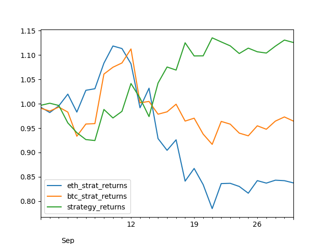
As can be seen from the plot above, even though both BTC and ETH went down, because the trader was correct in his assessment that BTC would outperform ETH , he still made a profit gross of fees (note fees would have been substantial through funding).
It is rather messy to calculate beta in the way we have done above, however, we can recognize that the slope of a linear regression is equivalent to the following where \(r\) represents the asset returns.
\(\beta = \frac{\text{Cov}(r_{eth}, r_{btc})}{\text{Var}(r_{btc})} \)
With this we can calculate beta for many assets at once using the covariance matrix, remembering the the diagonal of a covariance matrix is represents the asset's variance i.e. covariance with itself.
returns.cov() / np.diag(returns.cov())


'''

            BTCUSDT   ETHUSDT   BNBUSDT  ...   SOLUSDT   DOTUSDT   LTCUSDT
BTCUSDT    1.000000  0.670405  0.685812  ...  0.314637  0.484015  0.580629
ETHUSDT    1.116726  1.000000  0.921500  ...  0.442172  0.662352  0.753289
BNBUSDT    0.880659  0.710376  1.000000  ...  0.356652  0.567824  0.620400
XRPUSDT    0.959648  0.765593  0.833945  ...  0.388451  0.618470  0.711025
ADAUSDT    1.049320  0.829412  0.916797  ...  0.447160  0.693688  0.781825
DOGEUSDT   1.064683  0.861701  0.918580  ...  0.425492  0.641732  0.764610
MATICUSDT  1.357299  1.132466  1.231582  ...  0.591165  0.861791  0.952876
SOLUSDT    1.349409  1.138454  1.191177  ...  1.000000  0.882456  0.955674
DOTUSDT    1.158018  0.951340  1.057957  ...  0.492284  1.000000  0.849280
LTCUSDT    1.093428  0.851617  0.909833  ...  0.419631  0.668477  1.000000
'''


for sym in symbols:
    result = linregress(returns.BTCUSDT.values, returns[sym].values)
    print(f'Beta for {sym} regressed on btc is {result.slope}')

'''
Beta for BTCUSDT regressed on btc is 1.0
Beta for ETHUSDT regressed on btc is 1.1167261335021441
Beta for BNBUSDT regressed on btc is 0.8806586058262923
Beta for XRPUSDT regressed on btc is 0.9596483199266936
Beta for ADAUSDT regressed on btc is 1.0493203941766702
Beta for DOGEUSDT regressed on btc is 1.064683136297938
Beta for MATICUSDT regressed on btc is 1.357299269004374
Beta for SOLUSDT regressed on btc is 1.34940937776652
Beta for DOTUSDT regressed on btc is 1.1580180683203767
Beta for LTCUSDT regressed on btc is 1.0934283921870849
'''
The table below shows the beta for each asset pairing. I will leave it to the reader to expirement with backtesting different pairs at on different time horizons. Perhaps thinking about the fundamental reasons why the results are good or bad could provide some insight in how to effectively carry out strategies of this nature in the future.
| BTCUSDT | ETHUSDT | BNBUSDT | XRPUSDT | ADAUSDT | DOGEUSDT | MATICUSDT | SOLUSDT | DOTUSDT | LTCUSDT | |
|---|---|---|---|---|---|---|---|---|---|---|
| BTCUSDT | 1.000000 | 0.670405 | 0.685812 | 0.505653 | 0.516112 | 0.400757 | 0.391993 | 0.314637 | 0.484015 | 0.580629 |
| ETHUSDT | 1.116726 | 1.000000 | 0.921500 | 0.671966 | 0.679540 | 0.540290 | 0.544800 | 0.442172 | 0.662352 | 0.753289 |
| BNBUSDT | 0.880659 | 0.710376 | 1.000000 | 0.564261 | 0.579044 | 0.443997 | 0.456739 | 0.356652 | 0.567824 | 0.620400 |
| XRPUSDT | 0.959648 | 0.765593 | 0.833945 | 1.000000 | 0.700035 | 0.512869 | 0.504259 | 0.388451 | 0.618470 | 0.711025 |
| ADAUSDT | 1.049320 | 0.829412 | 0.916797 | 0.749936 | 1.000000 | 0.557217 | 0.544970 | 0.447160 | 0.693688 | 0.781825 |
| DOGEUSDT | 1.064683 | 0.861701 | 0.918580 | 0.717936 | 0.728113 | 1.000000 | 0.528237 | 0.425492 | 0.641732 | 0.764610 |
| MATICUSDT | 1.357299 | 1.132466 | 1.231582 | 0.920008 | 0.928123 | 0.688473 | 1.000000 | 0.591165 | 0.861791 | 0.952876 |
| SOLUSDT | 1.349409 | 1.138454 | 1.191177 | 0.877830 | 0.943263 | 0.686889 | 0.732226 | 1.000000 | 0.882456 | 0.955674 |
| DOTUSDT | 1.158018 | 0.951340 | 1.057957 | 0.779679 | 0.816313 | 0.577925 | 0.595472 | 0.492284 | 1.000000 | 0.849280 |
| LTCUSDT | 1.093428 | 0.851617 | 0.909833 | 0.705533 | 0.724164 | 0.541992 | 0.518240 | 0.419631 | 0.668477 | 1.000000 |
Pros and Cons of Long-Short Strategy
Pros:
- Can provide returns in both up and down markets: By taking both long and short positions, a long-short strategy can potentially generate positive returns in both bullish and bearish market conditions.
- May provide diversification benefits: Long-short strategies can diversify an investment portfolio by using a different investment approach than traditional "long-only" strategies.
- Can potentially reduce overall portfolio risk: The use of short positions can potentially help to reduce overall portfolio risk by hedging against market downturns.
Cons:
- Can be more complex: Long-short strategies are typically more complex than traditional investment strategies, requiring additional expertise and analysis to implement effectively.
- May require higher transaction costs: Because long-short strategies involve both long and short positions, they can involve higher transaction costs than traditional "long-only" strategies.
- Can be more volatile: While long-short strategies can potentially reduce overall portfolio risk, they can also be more volatile in the short-term due to the use of short positions. This increased volatility can make it more difficult to stick to an investment strategy during market fluctuations.
Data Collection Functions
def format_data(response):
    '''


    Parameters
    ----------
    respone : dict
        response from calling get_klines() method from pybit.
    freq : str
        DESCRIPTION.
        interval that has been passed in to get_klines method, used in order
        to round the datetimes, which will be mapped to pandas freq str

    Returns
    -------
    dataframe of ohlc data with date as index

    '''
    data = response.get('list', None)

    if not data:
        return

    data = pd.DataFrame(data,
                        columns =[
                            'timestamp',
                            'open',
                            'high',
                            'low',
                            'close',
                            'volume',
                            'turnover'
                            ],
                        )

    f = lambda x: dt.datetime.utcfromtimestamp(int(x)/1000)
    data.index = data.timestamp.apply(f)
    return data[::-1].apply(pd.to_numeric)

def get_last_timestamp(df):
    return int(df.timestamp[-1:].values[0])


def get_all_data(sym, interval):

    start = int(dt.datetime(2020, 1, 1).timestamp()* 1000)
    df = pd.DataFrame()
    while True:
        response = session.get_kline(category='linear',
                                     symbol=sym,
                                     start=start,
                                     interval=interval).get('result')

        latest = format_data(response)

        if not isinstance(latest, pd.DataFrame):
            break

        start = get_last_timestamp(latest)

        time.sleep(0.1)

        df = pd.concat([df, latest])
        print(f'Collecting data starting {dt.datetime.fromtimestamp(start/1000)}')
        if len(latest) == 1: break

    return df