Bollinger Bands with Python

Are you looking to take your cryptocurrency trading to the next level? Look no further than Bybit, the leading crypto derivatives exchange. With advanced trading tools, low fees, and a user-friendly platform, Bybit makes it easy to trade Bitcoin, Ethereum, and other popular cryptocurrencies. And if you sign up using our affiliate link  and use the referral code CODEARMO, you'll receive exclusive benefits and bonuses up to $30,000 to help you get started. Don't miss out on this opportunity to join one of the fastest-growing communities in crypto trading. Sign up for Bybit today and start trading like a pro!

 

 

To follow along with this tutorial you will need pandas and pandas_ta library installed. 

1. Open your command prompt or terminal.
2. Make sure you have Python 3 installed on your machine. You can check by typing python --version in your command prompt or terminal.
3. Install pandas_ta by typing pip install pandas_ta in your command prompt or terminal.
4. Once the installation is complete, you can import pandas_ta in your Python code by adding import pandas_ta at the top of your file.

 

 

 

What are Bollinger Bands?

 

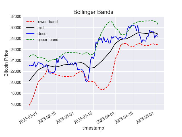
Bollinger Bands is a popular technical analysis tool used by traders to identify potential breakouts in price and analyze price volatility. It is composed of three lines - a moving average line, an upper band, and a lower band. The upper and lower bands are usually set two standard deviations away from the moving average line. The moving average line serves as a benchmark for the stock or asset's price action, while the upper and lower bands act as support and resistance levels.

Traders often use Bollinger Bands to determine whether an asset is overbought or oversold. When prices approach the upper band, it suggests that the asset may be overbought and due for a correction, while prices near the lower band suggest that the asset may be oversold and due for a rebound. Some traders use Bollinger Bands to identify entry and exit points for their trades, with a potential long trade being signaled when the price moves below the lower band and a potential short trade when the price moves above the upper band. Overall, Bollinger Bands is a powerful tool that can be used in combination with other indicators to make more informed trading decisions.

 

As can be seen from the plot below, these numbers are dynamic, a larger distance between the mid and the bands indicates higher volatility. Lower bandwidth would signify a quieter market.

 

Formulae for the upper, middle, and lower bands of the Bollinger Bands:

• Upper Band: \(UpperBand = MA + K\cdot\sigma\)
• Middle Band: \(MiddleBand = MA\)
• Lower Band: \(LowerBand = MA - K\cdot\sigma\)

Where:

• MA is the moving average
• K is the number of standard deviations from the mean (typically set to 2)
• \(\sigma\) is the standard deviation

 

 

Data Collection 

 

For the purpose of this article, we will utilize daily BTCUSDT data. The data collection code will be replicated from this article. The Bollinger Bands will be computed using daily data to ensure ease of analysis. However, should there be a preference for a different time interval, the linked article can be consulted to make the necessary adjustments.

 

from pybit.unified_trading import HTTP
import pandas as pd
import pandas_ta as ta
import numpy as np
import matplotlib.pyplot as plt
import datetime as dt
import json
import time

with open('authcreds.json') as j:
        creds = json.load(j)
        

key = creds['KEY_NAME']['key']
secret = creds['KEY_NAME']['secret']
  
session = HTTP(api_key=key, api_secret=secret, testnet=False)


def get_last_timestamp(df):
    return int(df.timestamp[-1:].values[0])

def format_data(response):
    '''
    

    Parameters
    ----------
    respone : dict
        response from calling get_klines() method from pybit.

    Returns
    -------
    dataframe of ohlc data with date as index

    '''
    data = response.get('list', None)
    
    if not data:
        return 
    
    data = pd.DataFrame(data,
                        columns =[
                            'timestamp',
                            'open',
                            'high',
                            'low',
                            'close',
                            'volume',
                            'turnover'
                            ],
                        )
    
    f = lambda x: dt.datetime.utcfromtimestamp(int(x)/1000)
    data.index = data.timestamp.apply(f)
    return data[::-1].apply(pd.to_numeric)



start = int(dt.datetime(2020, 1, 1).timestamp()* 1000)

interval = 'D'
symbol = 'BTCUSDT'
df = pd.DataFrame()

while True:
    response = session.get_kline(category='linear', 
                                 symbol=symbol, 
                                 start=start,
                                 interval=interval).get('result')
    
    latest = format_data(response, interval)
    
    if not isinstance(latest, pd.DataFrame):
        break
    
    start = get_last_timestamp(latest)
    
    time.sleep(0.1)
    
    df = pd.concat([df, latest])
    print(f'Collecting data starting {dt.datetime.fromtimestamp(start/1000)}')

 

 

Calculating Bollinger Bands

 

After collecting the data, the next step is to calculate the Bollinger Bands. This can be done easily with the pandas_ta module, as demonstrated below. For this calculation, we have used a moving average length of 20 days along with a multiplier of 2. However, it is important to note that these parameters can be adjusted based on individual preferences and requirements. By experimenting with these parameters, users can obtain more insight and potentially more accurate results.

 

df[['lower_band', 'mid', 'upper_band' ]] = ta.bbands(df.close, length=20, std=2).iloc[:, :3]

print(df[-1:][['lower_band', 'mid','close' , 'upper_band' ]])
'''
              lower_band       mid    close    upper_band
timestamp                                                
2023-05-03  26936.981086  28753.09  28472.4  30569.198914
'''

 

 

Visualize Bollinger Bands

 

In the following section, we generate signals for both long and short positions based on the calculated Bollinger Bands. A short signal is triggered when the Bitcoin closing price is greater than the upper band, while a long signal is generated when the closing price falls below the lower band. This is because the Bollinger Bands strategy is based on mean reversion, which implies that prices are likely to revert to their mean after deviating too far from it. In this case, the mean is represented by the 14-day moving average.

 

df['short_signal'] = np.where(df.close > df.upper_band, 1, 0)
df['long_signal'] = np.where(df.close < df.lower_band, 1, 0)

## lets plot the most recent 100 days
df[['lower_band', 'mid', 'close', 'upper_band']].plot(style=['k--', 'k-', 'b-', 'k--'])

plt.plot(df[df.long_signal==1]['close'], '^g')
plt.plot(df[df.short_signal==1]['close'], 'vr')
plt.title('Bollinger Bands Entries')
plt.ylabel('BTC Price USDT')

 

 

 

 

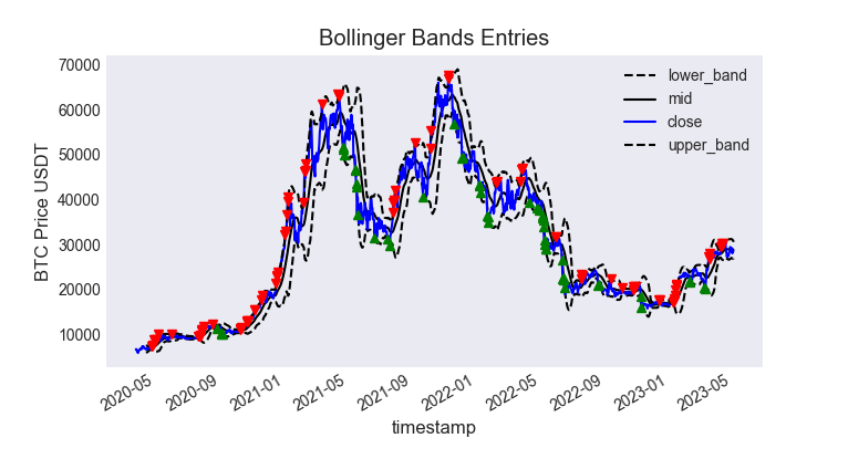
The Bollinger Bands demonstrated above generated sell signals throughout the bullish trend of 2021, leading to substantial losses for those who blindly followed the strategy. This is because in a trending market, such as the one observed in 2021, the price tends to surpass the upper band frequently, and the opposite for a bear market.

As an exercise, readers can explore enhancing the above strategy by incorporating a filter, such as taking long positions only if it aligns with a longer-term trend.

On the other hand, if a trader believes that the market is currently downwards trading, he may want to short when the upper band is reached as a potential way to make money in a bear market.