Vectors norms are a very important concept in machine learning. In a slightly unorthodox way, we will show the intuition behind this concept. In order to do this we will generate a large number of random vectors in two dimensions known as R2.
The following Python functions creates random vectors and plots them:
import matplotlib.pyplot as plt
import numpy as np
plt.style.use('seaborn-whitegrid')


def random_vector2d(n):
    x = np.linspace(-10,10,n)+np.random.uniform(-10,10,size=n)
    y = np.linspace(-10,10,n)+np.random.uniform(-10,10,size=n)
    vecs = [np.array([i,j]) for i,j in zip(x,y)]
    return vecs


def plot_vector2d(vector2d, ax, color=np.random.random(3),**options):
    return ax.arrow(0, 0, vector2d[0], vector2d[1],
              head_width=0.3, head_length=0.3,
              length_includes_head=True,color=color,**options)
Create and display 1000 random vectors
n= 1000
vecs = random_vector2d(n)

fig,ax =plt.subplots(figsize=(13,8))
for vec in vecs:
    plot_vector2d(vec,ax=ax,color=np.random.random(3),linewidth=4)

plt.axis([-20,20, -20, 20])
plt.axis('off')
plt.title('Random Vectors in $\mathbb{R}^2$',fontsize=20)
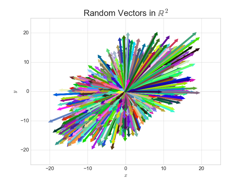
So although we have constrained the length of these vectors, notice that they can hit any point in \(\mathbb{R}^2\) if we were to multiply them by a scalar. As the title suggests, we are going to normalize these vectors and inspect the resulting shape.
L2 norm.
The L2 norm is simply the length/magnitude of a vector. The formula for calculating it is given below:
\(\||\vec{v}||_2=\Big(\sum\limits_{i=1}^{n}|\vec{v}_i|^2\Big)^{\frac{1}{2}}\)
Recalling the formula for the length of a 2d vector \(||\vec{v}|| = \sqrt{x^2+y^2}\) notice the formula above returns exactly the same answer since \(\sqrt{x} = x^{\frac{1}{2}}\)
In Python we can calculate this norm using the following function:
def l2_norm(vector):
    return (np.sum([i**2 for i in vector]))**(1/2)
L2 Normalized Vectors
A normalized vector will have a length of 1 and is often referred to as the unit vector. The formula to normalize a vector is given below:
\(\hat{v} = \frac{\vec{v}}{||\vec{v}||_2}\)
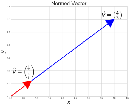
Example
Take the following vector \(\vec{v}\)
\(\vec{v} = \begin{bmatrix} 4 \\ 3 \\ \end{bmatrix} \hspace{0.5cm} \)
Calculate The L2 norm
\(||\vec{v}||_2 = \sqrt{4^2 + 3^2} = \sqrt{25} = 5\)
Calculate the L2 Normalized Vector
\(\hat{v} = \begin{bmatrix} \frac{4}{ \sqrt{4^2 + 3^2}} \\ \frac{3}{ \sqrt{4^2 + 3^2}} \\ \end{bmatrix} = \begin{bmatrix} \frac{4}{ 5} \\ \frac{3}{5} \\ \end{bmatrix} \)
Check the length of the resulting vector is 1
\(x^2 + y^2 =1\)
\((\frac{4}{5})(\frac{4}{5}) + (\frac{3}{5})(\frac{3}{5}) = \frac{16}{25} + \frac{9}{25} = \frac{25}{25} = 1\)
What does that look like?
The word norm is derived from the Latin normalis "in conformity with rule". In order to discover the rule behind this normalization process we will normalize the random vectors we created at the beginning on the document and plot them.
#normalizing vectors
l2_normed_vecs = [vec/l2_norm(vec) for vec in vecs]

fig,ax =plt.subplots(figsize=(9,6))
for vec in l2_normed_vecs:
    plot_vector2d(vec,ax=ax,color=np.random.random(3),linewidth=0.1)

plt.axis([-2,2, -2, 2])
plt.title('L2  Normalized Vectors',fontsize=20)
plt.xlabel("$x$",fontsize=25)
plt.ylabel("$y$",fontsize=25)
Clearly a pattern emerges when we calculate the L2 normalized vectors as shown below:
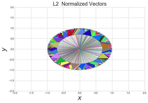
What rules can we derive from this?
1) When we normalize a vector \(\vec{v} \) the normalized vector \(\hat{v}\) will have a length of 1.
2) The Normalized vector will have the same direction as the original vector.
3) When thinking of L2 normalization in 2 dimensions, we should think: unit circle
L1 Norm
The L1 norm also known as the taxi-cab norm or the Manhattan norm. Is another common way to normalize vectors. The formula is given below:
\(||\vec{v}||_1 =\Big(\sum\limits_{i=1}^{n}|\vec{v}_i|^1\Big)^{\frac{1}{1}}\)
It may be slightly perplexing why the \(\frac{1}{1}\) exponent has been included in the formula above. However, it will soon become clear. Note that we could just as easily have written the formula above as:
\(||\vec{v}||_1 = \sum\limits_{i=1}^{n}|\vec{v}_i| \)
Python function for L1 norm
def l1_norm(vec):
    return np.sum([np.abs(i) for i in vec])
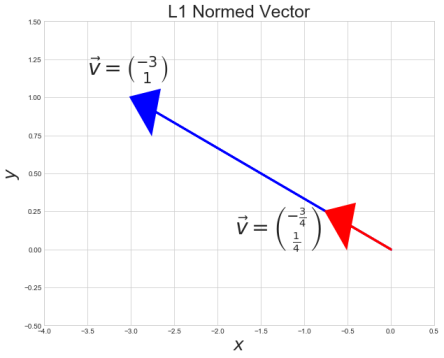
Example
Take the following vector \(\vec{v}\)
\(\vec{v} = \begin{bmatrix} -3 \\ 1 \\ \end{bmatrix} \hspace{0.5cm} \)
Take the L1 norm
\(||\vec{v}||_1 = (|x|^1 + |y|^1)^\frac{1}{1} = |x| + |y|\)
\(4 = |-3| + |1|\)
Normalize the vector by the L1 norm
\(\hat{v} = \begin{bmatrix} \frac{3}{( |-3|+|1|)} \\ \frac{3}{( |-3|+|1|)} \\ \end{bmatrix} = \begin{bmatrix} \frac{-3}{4} \\ \frac{1}{4} \\ \end{bmatrix} \)
Check the L1 norm of the resulting vector equals 1
\(|x| + |y| =1\)
\(|-\frac{3}{4}| + |\frac{1}{4}| = \frac{4}{4} = 1\)
What does that look like?
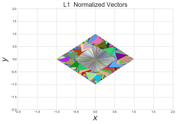
Let's normalize the random vectors we created at the beginning of the document using the L1 norm and inspect the resulting shape.
#normalizing vectors
l1_normed_vecs = [vec/l1_norm(vec) for vec in vecs]

fig,ax =plt.subplots(figsize=(9,6))
for vec in l1_normed_vecs:
    plot_vector2d(vec,ax=ax,color=np.random.random(3),linewidth=0.1)

plt.axis([-2,2, -2, 2])
plt.title('L1  Normalized Vectors',fontsize=20)
plt.xlabel("$x$",fontsize=25)
plt.ylabel("$y$",fontsize=25)
As with the L2 norm we see an nice shape emerge after normalizing the vectors. Whereas the L2 norm vectors produced a circle, the L1 shows a diamond.
What can we say about the L1 norm?
1) The L1 norm will always be greater than or equal to the L2 norm. Why? Think back to the fact that the L1 norm is also known as the taxicab norm, we could think of the L2 norm as the as the crow flies distance, whereas the L1 norm is equivalent to taking a taxi along streets that requires turns.
2) When we normalize a 2d vector by the L1 norm. The resulting vector's elements \(|x| + |y| = 1\)
3) When thinking of the L1 norm in 2d we should think of a diamond
In this section we will compare the formulae for the L1 and L2 norm. Recall the formula for the L1 norm for which a seemingly unnecessary exponents were included. Observe the formulae for the L1 and L2 norm below:
\(||\vec{v}||_1 = \Big(\sum\limits_{i=1}^{n}|\vec{v}_i|^1\Big)^{\frac{1}{1}} \\[5pt] ||\vec{v}||_2 = \Big(\sum\limits_{i=1}^{n}|\vec{v}_i|^2\Big)^{\frac{1}{2}} \\[5pt] \)
You may notice a pattern. Although Let's add one more to show the pattern:
\(||\vec{v}||_3 = \Big(\sum\limits_{i=1}^{n}|\vec{v}_i|^3\Big)^{\frac{1}{3}} \\[5pt] \)
The P-Norm
Hopefully the pattern has become clear, we simply take each element of the vector to the pth power. We can show a general formula for the norms we have so far:
\(||\vec{v}||_p = \Big(\sum\limits_{i=1}^{n}|\vec{v}_i|^p\Big)^{\frac{1}{p}} , \hspace{00.5cm}\text{for}\ p \geq 1\)
Infinity Norm
Clearly there are too many norms for us to show the shapes we would get from normalizing by the all the possibly integers. However, we can still get an idea for what they may look like. Consider what would happen if we increased p towards infinity.
\(||\vec{v}||_\infty = \underset{i\leq1\leq n}{max} \hspace{0.2cm} |\vec{v}_i|\)
The resulting norm is known as the infinity norm. It may not be clear how exactly we got from the formula for the p-norm to just taking absolute value from a vector. To understand why this is true, consider taking the elements of the a 2d vector and consider taking said elements to the power of \(p\), as \(p\) gets very large the larger of the two elements will begin to dominate the calculation.
Examples
Take the following vectors and find the infinity norms for each.
\(\vec{v} = \begin{bmatrix} -4 \\ 3\\ \end{bmatrix} \hspace{0.5cm} \vec{u} = \begin{bmatrix} -10 \\ 20\\ \end{bmatrix} \hspace{0.5cm} \vec{w} = \begin{bmatrix} 25 \\ 40\\ \end{bmatrix} \hspace{0.5cm}\\[20pt] ||\vec{v}||_\infty = 4 \hspace{0.5cm} ||\vec{u}||_\infty =20 \hspace{0.5cm} ||\vec{w}||_\infty = 40 \hspace{0.5cm}\)
So clearly the infinity norm is the easiest to calculate of all the norms we have considered so far, although it does require more thinking to get a grasp of it!
To normalize a vector by the infinity norm, we would simply divide the vector elements by the maximum absolute value. Lets take v from above as an example:
\(\vec{v} = \begin{bmatrix} \frac{-4}{4} \\ \frac{3}{4}\\ \end{bmatrix} = \begin{bmatrix} -1 \\ 0.75\\ \end{bmatrix}\)
Infinity norm in Python
def infinity_norm(vec):
    return np.max([abs(i) for i in vec])
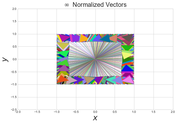
Normalize and plot the random vectors we have been working with:
inf_norm_vecs = [vec/infinity_norm(vec) for vec in vecs]

fig,ax =plt.subplots(figsize=(9,6))
for vec in inf_norm_vecs:
    plot_vector2d(vec,ax=ax,color=np.random.random(3),linewidth=0.1)

plt.axis([-2,2, -2, 2])
plt.title(r'$\infty$  Normalized Vectors',fontsize=20)
plt.xlabel("$x$",fontsize=25)
plt.ylabel("$y$",fontsize=25)
If there is nothing else you take away from this article, just remember the following:
L1 norm: Diamond
L2 norm: Circle
Infinity norm: Square