A good grasp of vectors is essential for mastering machine learning. This article will present a number of simple vector operations culminating in an applied example. Vectors are the prevalent in a number of fields. However, for the purposes of this article we will focus on their application in machine learning.
Article Contents:
- What is a vector?
- Vector operations
- Vector lengths and distances
- An applied example in machine learning KNN
What is a Vector?
A definition from lexico.com below:
"A quantity having direction as well as magnitude, especially as determining the position of one point in space relative to another."
Let's focus on the point "determining the position of one point in space relative to another" which is quite straightforward to interpret geometrically. An example of a two dimensional vector is given below:
\(\text{2d vector} = \begin{bmatrix} x \\ y \\ \end{bmatrix} \)
Note that the dimensionality of a vector relates to the number of elements it contains.
A two dimensional vector will have an \(x \) and \(y\) component. Vectors are often written with a \(\vec{}\) arrow accent indicating we are dealing with a vector therefore the above would become \(\vec{v}= \begin{bmatrix} x \\ y \\ \end{bmatrix} \)
In order to visualize what a two dimensional vector looks like, take two examples below.
\(\vec{v}_1 = \begin{bmatrix} 1 \\ 2 \\ \end{bmatrix} , \vec{v}_2 = \begin{bmatrix} 3 \\ 1 \\ \end{bmatrix} \)
Representing these vectors in Python:
import matplotlib.pyplot as plt
import numpy as np
plt.style.use('seaborn-whitegrid')

v1 = np.array([1,2])
v2 = np.array([3,1])
A helper function to visualize these vectors:
def plot_vector2d(vector2d, ax, color=np.random.random(3),**options):
    return ax.arrow(0, 0, vector2d[0], vector2d[1],
              head_width=0.3, head_length=0.3,
              length_includes_head=True,color=color,**options)
Plotting the two example vectors.
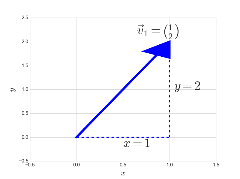
When seeing a two dimensional vector we should think of the first component as the \(x\) direction and the second component as the \(y\) direction. Therefore, for \(\vec{v}_1\) we move 1 unit in the \(x\) direction and two units in the \(y\) direction.
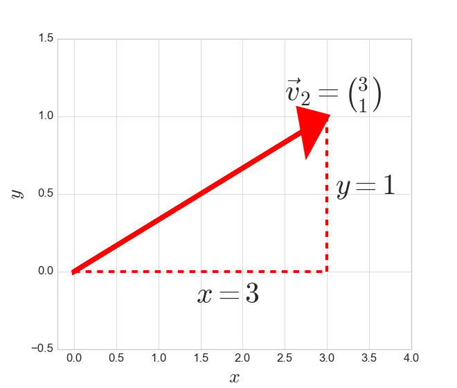
For \(\vec{v}_2\) we observe a move in the \(x\) direction of 3 units and a 1 unit move in the \(y\) direction.
Elementary Vector Operations
We can extend the notion of elementary operations in algebra to vectors. Vectors addition, subtraction and multiplication by a number are fairly straightforward.
Vector Addition
When we add two vectors, the result is a third vector. Taking the vectors we have been working with so far and adding them gives the following:
\(\vec{v}_1 = \begin{bmatrix} 1 \\ 2 \\ \end{bmatrix} ,\hspace{0.5cm} \vec{v}_2 = \begin{bmatrix} 3 \\ 1 \\ \end{bmatrix} ,\hspace{0.5cm} \vec{v}_3 = \vec{v}_1 + \vec{v}_2 = \begin{bmatrix} 1+3=4 \\ 2 +1=3\\ \end{bmatrix}\)
In Python:
v3 = v1+v2
print(v3)

Out:
array([4, 3])
Vector addition has a nice geometric interpretation as shown below. When adding two vectors, just picture lifting the tail of one vector and placing it at the head of the other. The \(\vec{v}_3 = \vec{v}_1 + \vec{v}_2\) which is represented by taking the tail (dashed blue line) and putting it at the head of the black vector which leads to a third vector illustrated by the red arrow.
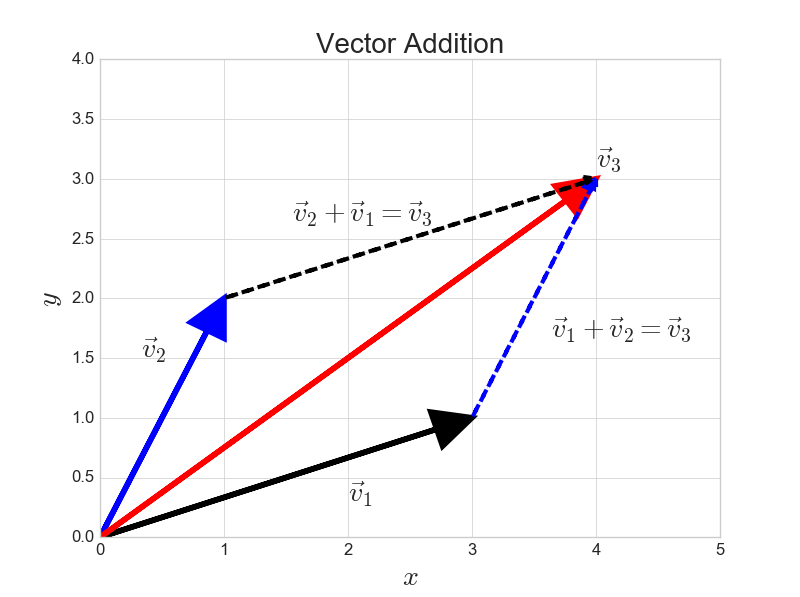
Notice above that we get the same answer regardless of whether we add \(\vec{v}_3 = \vec{v}_1 + \vec{v}_2\) or we add \(\vec{v}_3 = \vec{v}_2 + \vec{v}_1\) this property is true for all addition, the fact that the order we add vectors doesn't matter to the final outcome is known as commutivity.
Vector Subtraction
Vector subtraction works in a similar way, in that we just subtract the \(x\) and \(y\) components for each vector. As with vector addition, the result from this operation will be a new vector we will call \(\vec{v}_3\).
Subtracting \(\vec{v}_2 \) from \(\vec{v}_1\)
\(\vec{v}_1 = \begin{bmatrix} 1 \\ 2 \\ \end{bmatrix} ,\hspace{0.5cm} \vec{v}_2 = \begin{bmatrix} 3 \\ 1 \\ \end{bmatrix} ,\hspace{0.5cm} \vec{v}_3 = \vec{v}_1 - \vec{v}_2 = \begin{bmatrix} 1-3=-2 \\ 2 -1=1\\ \end{bmatrix}\)
v1 = np.array([1,2])
v2 = np.array([3,1])
v3 = v1-v2
v3

Out:
array([-2,  1])
Subtracting \(\vec{v}_1\) from \(\vec{v}_2\)
\(\vec{v}_1 = \begin{bmatrix} 1 \\ 2 \\ \end{bmatrix} ,\hspace{0.5cm} \vec{v}_2 = \begin{bmatrix} 3 \\ 1 \\ \end{bmatrix} ,\hspace{0.5cm} \vec{v}_3 = \vec{v}_2 - \vec{v}_1 = \begin{bmatrix} 3-1=2 \\ 1-2=-1\\ \end{bmatrix}\)
v3 = v2-v1
v3

Out:
array([ 2, -1])
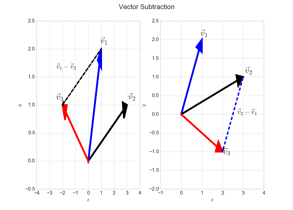
A geometric representation of vector subtraction is given below. The rule for vector subtraction, is that we flip the direction of the vector we are subtracting and put the tail at the head of the first vector. Notice when we subtract \(\vec{v}_2\ \text{from}\ \vec{v}_1\) as shown in the left plot, we flip the black vector \(\vec{v}_2\) upside-down and put it at the tip of the blue vector \(\vec{v}_1\) which then gives the new red colored vector.
Scalar Multiplication
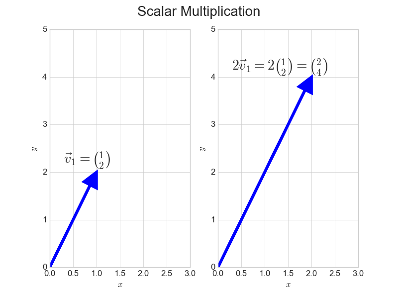
Consider a scalar to be just a real number for the purposes of this article. When we multiply a vector by a scalar, we simply multiply each element of the vector by the given scalar. Let's use our example vectors to demonstrate this concept.
Multiply the first vector by the scalar quantity 2.
\(2\vec{v}_1 = 2\begin{bmatrix} 1 \\ 2\\ \end{bmatrix} = \begin{bmatrix} 1\times 2 = 2\\ 2\times 2 = 4\\ \end{bmatrix}\)
v1*scalar1
Out:
 array([2, 4])
As we see in the plot below, multiplication by a scalar simply scales the vector elements. Notice the blue line on the right plot is twice the length as the one on the left prior to multiplication.
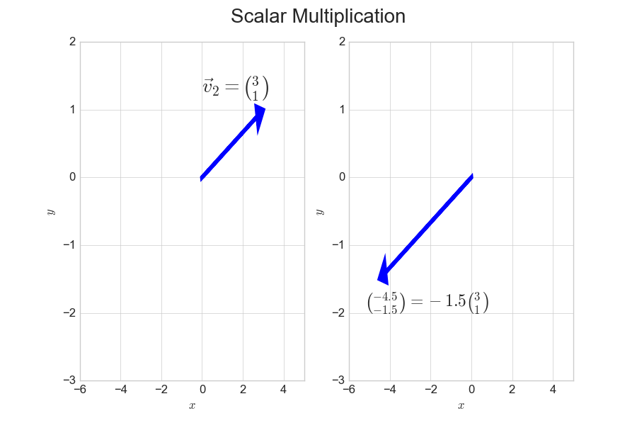
Multiplication by a negative scalar has a similar interpretation, in that the vector is scaled by the magnitude of the given scalar, but the direction is reversed.
\(-1.5\vec{v}_2 = -1.5\begin{bmatrix} 3 \\ 1\\ \end{bmatrix} = \begin{bmatrix} 3\times -1.5 = -4.5\\ 1\times -1.5 = -1.5\\ \end{bmatrix}\)
Length of a Vector
The length of a vector is also known as the magnitude or Euclidean norm depending on the context. In order to calculate the length of a 2d vector the following formula is used:
\(\text{length}\ \vec{v} = \sqrt{x^2 + y^2}\)
The general formula for the length of a n-dimensional vector is given below. Note that the \(i\) below denotes the index of the \(i^{th}\) element, therefore the first element would be \(x\) , the second would be \(y\) and the \(n^{th}\) element is the last element in the vector.
The length of a vector \(\vec{v}\) is denoted as \(||\vec{v}||\)
\(\text{length} = ||\vec{v}||= \sqrt{\sum\limits_{i=1}^{n} \vec{v}_i^2}, \hspace{0.5cm} \text{where}\ \vec{v} = \begin{bmatrix} v_1 \\ v_2 \\ \vdots\\ v_{n}\end{bmatrix}\)
To calculate this in Python we can use the function below:
def vector_length(vector):
    return np.sqrt(np.sum([i**2 for i in vector]))
A remind of the example vectors we have been using:
\(\vec{v}_1 = \begin{bmatrix} 1 \\ 2 \\ \end{bmatrix} , \vec{v}_2 = \begin{bmatrix} 3 \\ 1 \\ \end{bmatrix} \)
lv1 = vector_length(v1)
lv2 = vector_length(v2)
print(f"Length of v1: {lv1}")
print(f"Length of v2: {lv2}")

Out:
Length of v1: 2.23606797749979
Length of v2: 3.1622776601683795
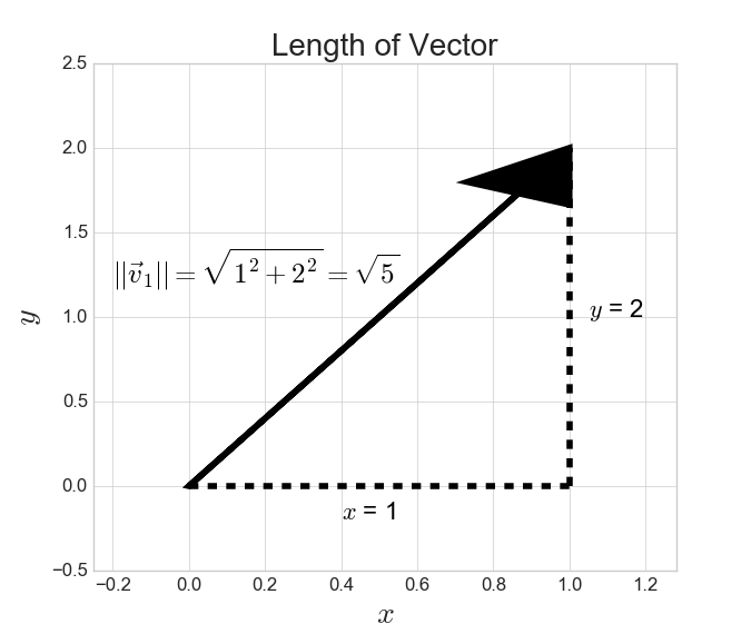
Taking the length of \(\vec{v}_1\) and showing the geometric interpretation below, we observe that the length of the vector is \(\sqrt{5}\) which agrees with the output from the python function shown above. You may recognize this length as being the hypotenuse of a right angled triangle from Pythagoras' theorem.
Distance Between Vectors
Whilst on this section on the length of a vector it may be useful to consider the length between two vectors, know as the distance. The precise term for this quantity is the Euclidean distance. The formula for the 2 dimensional case is given below:
\(\text{distance}\ (d)= \sqrt{(x_2-x_1)^2 + (y_2-y_1)^2}\)
We could make a formula to generalize the formula above for an \(n\) dimensional vector. However, notice we already have the tools to calculate this distance. We can utilize vector subtraction which we have already discussed and then take the length of the resulting vector as follows:
\(d(\vec{v},\vec{u}) = ||\vec{v}- \vec{u}||\)
vector_length(v1-v2)

Out:
2.23606797749979
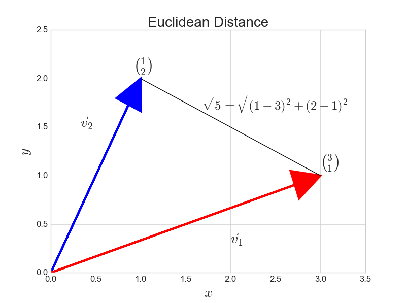
Let's check whether this result agrees with the result we got from Python. Note that although we used \(\vec{v}_1 -\vec{v}_2\) in the plot above, we would have gotten exactly the same answer we would have got from \(\vec{v}_2 - \vec{v}_1\) .
vector_length(v1-v2) == vector_length(v2-v1) == np.sqrt(5)

Out:
True
It should be said that there are other ways to calculate the distance between vectors, which we won't go into in this article.
What does all this have to do with machine learning?
The reader would be forgiven for being slightly lost as to how exactly these funny arrows on a graph relate to machine learning. In order to demonstrate the usefulness of vectors let's use the hello world of machine learning to put some of the math above into context.
K-Nearest-Neighbours
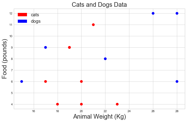
Let's say we have are given a dataset (made for illustrative purposes), of cats and dogs. We denote a cat by 0 and a dog by 1.
animals = np.array([0,1,0,0,1,0,1,0,1,0,1,0,1,0])
We have the following information about these animals in our dataset:
Weight: Animal weight in Kilograms (KG)
Food consumed per month: Weight of the food consumed in pounds.
weights = np.array([20, 15, 23, 17, 26, 18, 17, 20, 28, 19, 28, 21, 22, 19])
food_inpounds = np.array([6, 6, 4, 6, 12, 4, 9, 4, 6, 9, 12, 11, 8, 9])
On reflection these would be some very heavy cats. But onwards nonetheless!
Let's visualize our dataset:
colors = ['blue' if i ==1 else 'red' for i in animals]
fig,ax=plt.subplots(figsize=(10,6))
plt.scatter(weights, food_inpounds,60, c=colors)
plt.ylabel('Food (pounds)',fontsize=20)
plt.xlabel('Animal Weight (Kg)',fontsize=20)
plt.title("Cats and Dogs Data",fontsize=20)

import matplotlib.patches as mpatches

classes = ['cats','dogs']
class_colours = ['r','b']
recs = []
for i in range(0,len(class_colours)):
    recs.append(mpatches.Rectangle((0,0),1,1,fc=class_colours[i]))
plt.legend(recs,classes,loc='best',prop={'size': 15})
Say we get a new data-point and we know only the animals weight and food consumption. Can we make a prediction regarding whether its a cat or a dog based on what we know? We see the animal is 22 kg and eats 10 pounds of food per month.
new_point = np.array([22,10])
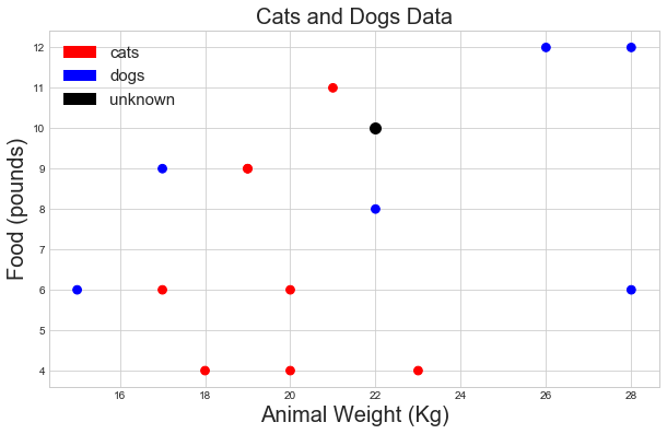
We are going to assume animals with the similar weights and food consumption are the more likely to be the same species. Therefore we are going to find the nearest neighbours to our unknown data point and classify the new point based on a majority vote between the them.
How many neighbours (k) should we use?
The number of neighbours is the k from the name of the algorithm. For the convenience we will use the 3 nearest neighbours to our unknown data point. Therefore k=3.
How do we define 'nearest' ?
Well clearly we can see from the plot above which points are the 3 nearest neighbours to our datapoint. However, bear in mind that we can't always plot data and look at it as we can in this contrived example.
You may realize that we can calculate the distance between the points, as we did in the 'distance between vectors' section. Let's plot the Euclidean Distance between the unknown point and the labeled data.
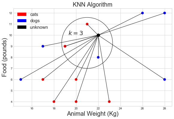
Looking at the above plot, it appears that the unknown point's 3 nearest neighbours and 2 cats and 1 dog. Therefore the KNN algorithm would predict that the unknown point is a cat, by a majority vote of 2:1.