This article series is provided by guest author James. It aims to help build an understanding of fixed income markets, securities, and interest rates through Python code.
In the previous article, I asked if yield was a good comparable return measure for security selection using two bonds:
| Bond | Maturity | Coupon | Price | Yield |
| A | 3-year | 6% | 99.33 | 6.25% |
| B | 7-year | 6% | 97.15 | 6.52% |
import yearfrac as yf
import matplotlib.pyplot as plt
import pandas as pd
from collections import namedtuple

t = list(range(1,8))
i = [5.0, 5.375, 6.25, 6.375, 6.5, 6.51, 6.52]

plt.figure(figsize = (20, 10))
plt.plot(t, i)
plt.title("Yield Curve", fontsize = 32)
plt.xlabel("Maturity(Years)", fontsize = 18)
plt.ylabel("Rate (%)", fontsize = 18)
plt.xticks(fontsize = 18)
plt.yticks(fontsize = 18)
plt.show()
Your holding period is one year and this is your interest rate environment (curve). We did not expect yields to change during the holding period:
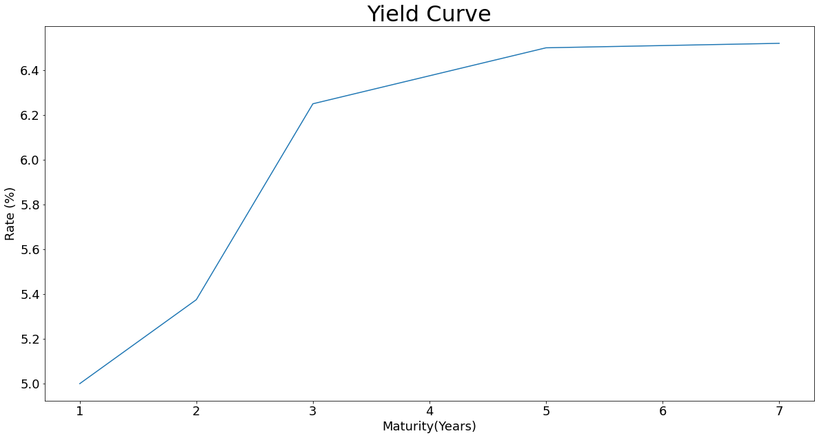
| Year | 1 | 2 | 3 | 4 | 5 | 6 | 7 |
| Yield | 5.000% | 5.375% | 6.250% | 6.375% | 6.500% | 6.510% | 6.520% |
Let's start by setting up our holding period dates and bond data. For now, we are going to manually edit the inputs, this may seem tedious, but it will help us identify the processes that we need to automate in our Python code later in this article.
First, we will define our holding period in terms of dates. The settlement date is our start date when we buy the bonds, the horizon date is exactly a year later which is when we will sell the bonds:
settlement_date = (2021, 9, 1)

horizon_date = (2022, 9, 1)
Here we are applying the bond price function for given a yield calculation, that we used in our previous article, I have just renamed the variable names.
bond_a_coupon_schedule_at_settle = [(2022, 9, 1),
                                    (2023, 9, 1),
                                    (2024, 9, 1)]

bond_a_at_settle = (bond_a_coupon_schedule_at_settle, 0.06, 1, 100, (2021, 9, 1))

bond_a_settle_px = bond_price(settlement_date,  *bond_a_at_settle, 0.0625)

bond_a_settle_px
To calculate the bond price at the horizon date we need to update the inputs:
- Remove the coupon date(s) that fall between the settlement and horizon date
- Update the previous coupon date
- Calculate the bond price using the horizon date as the settlement date and yields from our curve (one year has elapsed since we bought the three and seven year bonds)
bond_a_coupon_schedule_at_horizon = [(2023, 9, 1), (2024, 9, 1)]

bond_a_at_horizon = (bond_a_coupon_schedule_at_horizon, 0.06, 1, 100, (2022, 9, 1))

bond_a_horizon_px = bond_price(horizon_date,  *bond_a_at_horizon, 0.05375) #2-year yield

bond_a_horizon_px
We repeat the same steps for Bond B except that we use the 6-year yield.
Bond B data at settlement date:
bond_b_coupon_schedule_at_settle = [(2022, 9, 1),
                                    (2023, 9, 1),
                                    (2024, 9, 1),
                                    (2025, 9, 1),
                                    (2026, 9, 1),
                                    (2027, 9, 1),
                                    (2028, 9, 1)]

bond_b_at_settle = (bond_b_coupon_schedule_at_settle, 0.06, 1, 100, (2021, 9, 1))

bond_b_settle_px = bond_price(settlement_date, *bond_b_at_settle, 0.0652)

bond_b_settle_px
Bond B data at horizon date:
bond_b_coupon_schedule_at_horizon = [(2023, 9, 1),
                                     (2024, 9, 1),
                                     (2025, 9, 1),
                                     (2026, 9, 1),
                                     (2027, 9, 1),
                                     (2028, 9, 1)]

bond_b_at_horizon = (bond_b_coupon_schedule_at_horizon, 0.06, 1, 100, (2022, 9, 1))

bond_b_horizon_px = bond_price(horizon_date, *bond_b_at_horizon, 0.0651)# 6-year yield

bond_b_horizon_px
Comparing the price return of each bond during our holding period:
bond_a_price_return = bond_a_horizon_px / bond_a_settle_px -1
bond_b_price_return = bond_b_horizon_px / bond_b_settle_px -1

print(f'Bond A Price Return: {round(bond_a_price_return, 6) * 100}%')
print(f'Bond B Price Return: {round(bond_b_price_return, 6) * 100}%')
| Settlement Price | Horizon Price | Price Return | |
|---|---|---|---|
| Bond A | 99.335 | 101.156 | 1.833% |
| Bond B | 97.150 | 97.532 | 0.393% |
The return on Bond A was substantially higher because we are not operating on a flat interest rate curve. This effect is known as roll-down, since we are rolling down the curve to a lower yield instead of approaching maturity at a constant yield.
What if we are holding the bond to maturity, surely, we don't need to care about this? After all it is yield-to-maturity, right?
Another assumption of YTM (yield to maturity) is that we re-invest all received cash flows at YTM for the remaining life of the bond, another assumption that crumbles when we do not have a flat curve.
To calculate the return of holding a bond we must consider the yield at the horizon date and the rate at which we can reinvest the received cash flows until the horizon date. This is known as horizon rate return or total return analysis which we are going to explore in this article.
While building the code I will use our original Bond B and a holding period of two years.
Our bond B data:
settlement_date = (2021, 9, 1)
horizon_date = (2023, 9, 1)

bond_b_coupon_schedule = [(2022, 9, 1),
                          (2023, 9, 1),
                          (2024, 9, 1),
                          (2025, 9, 1),
                          (2026, 9, 1),
                          (2027, 9, 1),
                          (2028, 9, 1)]

bond_b = (bond_b_coupon_schedule, 0.06, 1, 100, (2021, 9, 1))
We want to identify all the coupon dates that fall between the settlement date and the horizon date. Previously, we had to go directly into the coupon schedule, identify and remove these manually:
def hpr_received_coupons(settlement_date, coupon_schedule, horizon_date):
    """
    This is a function which evaluates which coupon dates will be realised
    in a coupon schedule between a settlement and horizon date.

    INPUTS:
    # settlement_date = Single date value for the date at which the security
        is exchanged for cash, typically T+1 or T+2, iterable containing: YYYY, MM, DD

    # coupon_schedule = The dates of bonds cash flows where the first date is
        the next coupon date and the last is the maturity of the bond

    # horizon_date = Single date value when the bond will be transacted in
        the future

    OUTPUTS:
    # coupon_dates_within_holding_period = an iterable containing realised
        coupon dates
    """
    holding_period = yf.d30360e(*settlement_date, *horizon_date, matu = False)
    coupon_dates_within_holding_period = []

    for dates in coupon_schedule:
        if yf.d30360e(*settlement_date, *dates, matu = False) <= holding_period:
            coupon_dates_within_holding_period.append(dates)

    return coupon_dates_within_holding_period
Let's test the output using only the coupon schedule as of the settlement date, using the same bond data inputs as previous articles along with the horizon date.
The function successfully extracts the dates that fall between the settlement and horizon dates. These are inclusive, so if a coupon falls on the settlement date or/and horizon date then this a coupon that we have received.
hpr_received_coupons(settlement_date, bond_b_coupon_schedule, horizon_date)
Returns: [(2022, 9, 1), (2023, 9, 1)]
Next, we need to calculate the coupon amounts that we receive on the realised dates between the settlement and horizon dates but before that we need to update one of our original bond price calculation functions.
We are going to edit our original cash_flows function with an additional parameter that allows us to override and stop the principal amount being added to the final cash flow. By default, the principal is included so that we do not have to edit the entire bond price script.
def cash_flows(coupon_schedule,
               coupon_rate,
               coupon_freq,
               face,
               to_maturity = True):
    """
    This a function which models the cash flows amounts of the bond and
    outputs a list of nominal cash flows

    INPUTS:
    #coupon_schedule = the dates of bonds cash flows where the first date
        is the next coupon date and the last is the maturity of the bond

    #coupon_rate = the interest rate paid by the bond, expressed as
        a decimal value

    #coupon_freq =  the number of times per year that the bond
        pays interest

    #face =  the par amount of the bond

    UPDATE
    #to_maturity = Adds the bond principal to the final cash flow, this
        defaults to True.

    OUTPUTS:
    #cf = a list object containing nominal cash flows
    """
    cf = []

    for dates in coupon_schedule:
        cf.append(coupon_rate * face / coupon_freq)

    if to_maturity:
        cf[-1] += face

    return cf
We then apply the updated cash_flow function with the override, to_maturity enabled.
def hpr_coupon_amounts(settlement_date,
                        coupon_schedule,
                        horizon_date,
                        coupon_rate,
                        coupon_freq,
                        face):
    """
    This is a function which calculates the coupon amounts for realised coupons
        during the holding period.

    INPUTS:
    # settlement_date = Single date value for the date at which the security
        is exchanged for cash, typically T+1 or T+2, iterable containing: YYYY, MM, DD

    # coupon_schedule = The dates of bonds cash flows where the first date is
        the next coupon date and the last is the maturity of the bond

    # horizon_date = Single date value when the bond will be transacted in
        the future

    # coupon_rate = the interest rate paid by the bond, expressed as a decimal value

    # coupon_freq = the number of times per year that the bond pays interest

    # face =  the par amount of the bond

    OUTPUTS:
    # cf = an iterable containing realised coupon amounts
    """

    coupon_dates_within_holding_period = hpr_received_coupons(settlement_date,
                                                              coupon_schedule,
                                                              horizon_date)

    cf = cash_flows(coupon_dates_within_holding_period,
                    coupon_rate,
                    coupon_freq,
                    face,
                    to_maturity = False)

    return cf
Again we will test our function:
settlement_date = (2021, 9, 1)
horizon_date = (2023, 9, 1)

hpr_coupon_amounts(settlement_date, bond_b_coupon_schedule, horizon_date, 0.06, 1, 100)
Returns: [6.0, 6.0]
Great, now we can isolate the coupon dates and amounts from our original bond data frame for a given horizon date.
To calculate the total return, we are going to calculate the present value of the bond at the settlement date and the future value of the bond at the horizon date. The total return is then the percentage change between the present and future value which we will annualise.
The future value of the bond has two components: The price of the bond at the horizon date using the assumed future yield and the future value of all realised coupons reinvested at the reinvestment rate. How do we calculate the future value? It is the present value calculation that we explored in the first article but re-arranged to discount forward in time rather than back to present.
The original PV calculation:
\(PV=\frac{FV_{t}}{\left( 1+i_{t} \right)^{t}}\)
\( \text{where:}\)
\(PV=\text{Present value of cash flow}\)
\(FV=\text{Future value of cash flow}\)
\(t=\text{Time, years until receipt of cash flow }\)
\(i=\text{interest rate for time, t}\)
Re-arrange and express the terms of future value:
\(FV=PV_{t}\left( 1+i_{t} \right)^{t}\)
Now we are receiving time dependent, \(PV_{t} \) and these are discounted forward at a re-investment rate to find a single future value, \(\text{FV}\). We will use this calculation for our realised coupons, and it means that we are longer forced to accept the bond yield as the re-investment rate for our cash receipts.
Now we will construct a Python function, hpr_coupon_horizon_value to calculate this for us. It will first generate a list containing the investment period for each realised coupon, the time between each realised coupon date and the horizon date.
Using the investment periods and the re-investment rate we will calculate the discount factors for each coupon. Because we are discounting forward in time, these will be greater than one (assuming that the re-investment rate is greater than zero).
Each coupon is then multiplied with each coupon's respective discount factor, the sum of these products is then finally the future value of all realised coupons as of the horizon date.
def hpr_coupon_horizon_value(settlement_date,
                        coupon_schedule,
                        horizon_date,
                        coupon_rate,
                        coupon_freq,
                        face,
                        reinvestment_rate):
    """
    This is a function which calculates the future value of realised coupons
    at the horizon date and sums them.

    INPUTS:
    # settlement_date = Single date value for the date at which the security
        is exchanged for cash, typically T+1 or T+2, iterable containing: YYYY, MM, DD

    # coupon_schedule = The dates of bonds cash flows where the first date is
        the next coupon date and the last is the maturity of the bond

    # horizon_date = Single date value when the bond will be transacted in
        the future

    # coupon_rate = the interest rate paid by the bond, expressed as a decimal value

    # coupon_freq = the number of times per year that the bond pays interest

    # face =  the par amount of the bond

    # reinvestment_rate = the discount rate used to calculate future value
        of realised coupons

    OUTPUTS:
    # sum(fv_coupon) = the sum of future value of realised coupons
    """

    # a list to contain the time between each coupon date and the horizon date
    investment_periods = []

    # calculation of each time period
    for dates in hpr_received_coupons(settlement_date, coupon_schedule, horizon_date):
        investment_periods.append(yf.d30360e(*dates, *horizon_date, matu = False))

    # a list containing the discount factor for each coupon
    df = []

    # calculation of each discount factor
    for periods in investment_periods:
        df.append((1 + reinvestment_rate / coupon_freq) ** (periods * coupon_freq))

    # a function that generates a list containing each coupon amount
    cf = hpr_coupon_amounts(settlement_date,
                        coupon_schedule,
                        horizon_date,
                        coupon_rate,
                        coupon_freq,
                        face)

    # a lit comprehension that contains the future value of each coupon
    fv_coupon = [df[i] * cf[i] for i in range(len(cf))]

    # return value is the total sum of all coupon future values
    return sum(fv_coupon)
Based on the inputs in this example, we are calculating - Given that we are buying the bond on the 1st of September 2021 and holding the bond until the 1st of September 2023, what is the future value of the realised coupons, assuming a re-investment rate of 9%?
settlement_date = (2021, 9, 1)
horizon_date = (2023, 9, 1)

hpr_coupon_horizon_value(settlement_date, bond_b_coupon_schedule, horizon_date, 0.06, 1, 100, 0.09)
Returns: 12.540
The second component of the future value is the price of the bond at the horizon date at the assumed yield for that future date. Again, we want to write our function in a manner so that we do not have edit our underlying bond data. Instead, we want to give it the data that we have as of today and only provide the assumed yield.
This function is very similar to the bond_price function that we designed in the second article. However, here we can now enter the horizon date and the function will automatically update the coupon schedule and the previous coupon date.
def hpr_horizon_bond_price(settlement_date,
                           horizon_date,
                           coupon_schedule,
                           coupon_rate,
                           coupon_freq,
                           face,
                           prev_coupon,
                           bond_horizon_yld,
                           clean = True,
                           precision = 6):
    """
    This is a function which calculates the price of a bond at a future date, the horizon date.

    #INPUTS:
    # settlement_date = Single date value for the date at which the security
        is exchanged for cash, typically T+1 or T+2, iterable containing: YYYY, MM, DD

    # horizon_date = Single date value when the bond will be transacted in
        the future

    # coupon_schedule = The dates of bonds cash flows where the first date is
        the next coupon date and the last is the maturity of the bond

    # coupon_rate = the interest rate paid by the bond, expressed as a decimal value

    # coupon_freq = the number of times per year that the bond pays interest

    # face =  the par amount of the bond

    # prev_coupon =  an iterable that contains the date value, YYYY, MM, DD
        of when the previous coupon was paid

    # bond_horizon_yld = The yield at which the bond is being priced at the horizon date

    #clean = Boolean which defaults to True. When True the function returns
        the clean price of the bond, False it returns the dirty price of the bond.

    # precision = The number of decimals that the bond price will be calculated to,
        defaults to six

    OUTPUTS:
    #The price of the bond at the horizon date, in clean or dirty terms
        dependent on the function inputs.
    """

    # Generate a list containing the received coupons
    received_coupons = hpr_received_coupons(settlement_date, coupon_schedule, horizon_date)

    # Remove the recevied coupons from the coupon schedule
    remaining_coupons = [date for date in coupon_schedule
                                if date not in received_coupons]

    # Use the latest received coupon as the previous coupon date
    prev_coupon = received_coupons[-1]

    # Bond price calculated on the horizon date using the adjusted coupon schedule
    dirty_px = present_value(horizon_date, remaining_coupons, coupon_rate,
                             coupon_freq, face, bond_horizon_yld)

    # Accrued interest calculated as of the horizon date using the adjusted coupon schedule
    ai = accrued_interest(horizon_date, remaining_coupons, coupon_rate,
                          coupon_freq, face, prev_coupon)

    if clean:
        return round(dirty_px - ai, precision)
    else:
        return round(dirty_px, precision)
Based on the inputs in this example, we are calculating - What is the price of the bond assuming that we are settling it on the 1st of the September 2023 at an assumed yield of 6%? Because the assumed yield equals the coupon rate, the bond will be priced at par which is also reflected in our output.
settlement_date = (2021, 9, 1)
horizon_date = (2023, 9, 1)

hpr_horizon_bond_price(settlement_date, horizon_date, *bond_b, 0.06)
Returns: 100.000
Great! We now have the two components of the future value now we just need to combine them.
def hpr_total_future_value(settlement_date,
                    horizon_date,
                    coupon_schedule,
                    coupon_rate,
                    coupon_freq,
                    face,
                    prev_coupon,
                    bond_horizon_yld,
                    reinvestment_rate):

    """
    This is a function which combines the output from the bond_price_at_horizon_date
        and hpr_coupon_horizon_value to calculate the total future value of the bond
        at the horizon date.

    #INPUTS:
    # settlement_date = Single date value for the date at which the security
        is exchanged for cash, typically T+1 or T+2, iterable containing: YYYY, MM, DD

    # horizon_date = Single date value when the bond will be transacted in
        the future

    # coupon_schedule = The dates of bonds cash flows where the first date is
        the next coupon date and the last is the maturity of the bond

    # coupon_rate = the interest rate paid by the bond, expressed as a decimal value

    # coupon_freq = the number of times per year that the bond pays interest

    # face =  the par amount of the bond

    # prev_coupon =  an iterable that contains the date value, YYYY, MM, DD
        of when the previous coupon was paid

    # bond_horizon_yld = The yield at which the bond is being priced at the horizon date

    # reinvestment_rate = the discount rate used to calculate future value
        of realised coupons

    OUTPUTS:
    # The total future value of the bond, including reinvested coupons
    """

    bond_price_at_horizon_date = hpr_horizon_bond_price(
                    settlement_date,
                    horizon_date,
                    coupon_schedule,
                    coupon_rate,
                    coupon_freq,
                    face,
                    prev_coupon,
                    bond_horizon_yld)

    reinvested_coupons = hpr_coupon_horizon_value(settlement_date,
                        coupon_schedule,
                        horizon_date,
                        coupon_rate,
                        coupon_freq,
                        face,
                        reinvestment_rate)

    return bond_price_at_horizon_date + reinvested_coupons
Again, reading the inputs to understand what this function is answering - What is the future value at the horizon date when investing in bond B for two years assuming a horizon yield of 6% and a re-investment rate of 5%?
settlement_date = (2021, 9, 1)
horizon_date = (2023, 9, 1)

hpr_total_future_value(settlement_date, horizon_date, *bond_b, 0.06, 0.05)
Returns: 112.300
We now have the total future value of the bond and from the previous article we can calculate the present value of the bond. Now we just need to calculate the percentage change between the two, known as the holding period return which we will finally annualise.
\(\text{Holding Period Return} = \frac{FV}{PV}-1\)
\(\text{where:}\)
\(PV=\text{Present value of the bond}\)
\(FV=\text{Future value of the bond, including reinvested coupons}\)
\(\text{Annualised Return} = \left( 1 + \text{Holding Period Return} \right)^{\frac{1}{T}}-1\)
\(\text{where:}\)
\(T=\text{Time, years between settlement and horizon date}\)
def hpr_return(settlement_date,
               horizon_date,
               coupon_schedule,
               coupon_rate,
               coupon_freq,
               face,
               prev_coupon,
               bond_settle_yld,
               bond_horizon_yld,
               reinvestment_rate,
               return_hpr = False):

    """
    This is a function which calculates the total future value of the bond and the
    present value of the bond. It then evaluates the percentage change from present
    value to future value which is then annualised. The function also has the option
    to return the holding period return (non-annualised return).

    #INPUTS:
    # settlement_date = Single date value for the date at which the security
        is exchanged for cash, typically T+1 or T+2, iterable containing: YYYY, MM, DD

    # horizon_date = Single date value when the bond will be transacted in
        the future

    # coupon_schedule = The dates of bonds cash flows where the first date is
        the next coupon date and the last is the maturity of the bond

    # coupon_rate = the interest rate paid by the bond, expressed as a decimal value

    # coupon_freq = the number of times per year that the bond pays interest

    # face =  the par amount of the bond

    # prev_coupon =  an iterable that contains the date value, YYYY, MM, DD
        of when the previous coupon was paid

    # bond_settle_yld = The yield at which the bond is traded on the settlement day

    # bond_horizon_yld = The yield at which the bond is being priced at the horizon date

    # reinvestment_rate = the discount rate used to calculate future value
        of realised coupons

    # return_hpr = Boolean that defaults to False. If set to True the function
        will return the holding period return instead of the annualised return

    OUTPUTS:

    # The annualised return or holding period return of the bond for the holding
        period for the given settlement yield horizon yield and reinvestment rate.
    """

    fv = hpr_total_future_value(settlement_date,
                                horizon_date,
                                coupon_schedule,
                                coupon_rate,
                                coupon_freq,
                                face,
                                prev_coupon,
                                bond_horizon_yld,
                                reinvestment_rate)

    pv = bond_price(settlement_date,
                    coupon_schedule,
                    coupon_rate,
                    coupon_freq,
                    face,
                    prev_coupon,
                    bond_settle_yld)

    holding_period_return = fv / pv -1

    if return_hpr:
        return  holding_period_return

    holding_period = yf.d30360e(*settlement_date, *horizon_date, matu = True)

    annualised_return = (1 + holding_period_return) ** (1 / holding_period) - 1

    return annualised_return
We now have the ability to calculate the total return of buying Bond B at a yield of 6.52%, holding it for two years, sell it at an assumed yield 6.5% and a re-investment rate of 5%.
settlement_date = (2021, 9, 1)
horizon_date = (2023, 9, 1)

hpr_return(settlement_date, horizon_date, *bond_b, 0.0652, 0.065, 0.05)
Returns 0.0652 (6.52%)
Using different horizon yields and reinvestment rates we can construct two basic scenario analysis tables for a bond and a given horizon date.
For this analysis we will use Bond B again. It pays an annual coupon of 6% that matures 2028. We are trading the bond at a yield of 6.52% and our trade will settle on the 1st of September 2021. We intend to hold the bond for two years until 1st of September 2023.
settlement_date = (2021, 9, 1)
horizon_date = (2023, 9, 1)

bond_b_coupon_schedule = [(2022, 9, 1),
                          (2023, 9, 1),
                          (2024, 9, 1),
                          (2025, 9, 1),
                          (2026, 9, 1),
                          (2027, 9, 1),
                          (2028, 9, 1)]

# coupon dates, coupon rate, coupon freq, face, previous coupon
bond_b = (bond_b_coupon_schedule, 0.06, 1, 100, (2021, 9, 1))
We will first create a table containing tuples where the first element of each tuple is the re-investment rate and the second element is the horizon yield. These are the inputs that we will feed into the hpr_future_value and hpr_return functions.
index = ['3%', '4%','5%','6%','7%', '8%', '9%']
columns = ['3%', '4%', '5%', '6%', '7%', '8%','9%']

scenario_inputs = pd.DataFrame([
                    [(0.03, 0.03), (0.03, 0.04), (0.03, 0.05), (0.03, 0.06), (0.03, 0.07), (0.03, 0.08), (0.03, 0.09)],
                   [(0.04, 0.03), (0.04, 0.04), (0.04, 0.05), (0.04, 0.06), (0.04, 0.07), (0.04, 0.08), (0.04, 0.09)],
                   [(0.05, 0.03), (0.05, 0.04), (0.05, 0.05), (0.05, 0.06), (0.05, 0.07), (0.05, 0.08), (0.05, 0.09)],
                   [(0.06, 0.03), (0.06, 0.04), (0.06, 0.05), (0.06, 0.06), (0.06, 0.07), (0.06, 0.08), (0.06, 0.09)],
                   [(0.07, 0.03), (0.07, 0.04), (0.07, 0.05), (0.07, 0.06), (0.07, 0.07), (0.07, 0.08), (0.07, 0.09)],
                   [(0.08, 0.03), (0.08, 0.04), (0.08, 0.05), (0.08, 0.06), (0.08, 0.07), (0.08, 0.08), (0.08, 0.09)],
                   [(0.09, 0.03), (0.09, 0.04), (0.09, 0.05), (0.09, 0.06), (0.09, 0.07), (0.09, 0.08), (0.09, 0.09)]
                   ],columns = columns, index=index)
scenario_fv = scenario_inputs.applymap(lambda x: round(hpr_total_future_value(settlement_date,
                                                                        horizon_date,
                                                                        *bond_b,
                                                                        x[1], # horizon yield
                                                                        x[0] # re-investment rate
                                                                       ),4)) #rounded to 4 dp

scenario_fv
The total future value of of Bond B at the horizon date:
| Horizon Yield | ||||||||
| 3% | 4% | 5% | 6% | 7% | 8% | 9% | ||
|
Reinvestment Rate |
3% | 125.919 | 121.084 | 116.510 | 112.180 | 108.080 | 104.195 | 100.511 |
| 4% | 125.979 | 121.144 | 116.570 | 112.240 | 108.140 | 104.255 | 100.571 | |
| 5% | 126.039 | 121.204 | 116.630 | 112.300 | 108.200 | 104.315 | 100.631 | |
| 6% | 126.099 | 121.264 | 116.690 | 112.360 | 108.260 | 104.375 | 100.691 | |
| 7% | 126.159 | 121.324 | 116.750 | 112.420 | 108.320 | 104.435 | 100.751 | |
| 8% | 126.219 | 121.384 | 116.810 | 112.480 | 108.380 | 104.495 | 100.811 | |
| 9% | 126.279 | 121.444 | 116.870 | 112.540 | 108.440 | 104.555 | 100.871 | |
scenario_returns = scenario_inputs.applymap(lambda x: str(round(100 *hpr_return(settlement_date,
                                                                 horizon_date,
                                                                 *bond_b,
                                                                 0.0652,
                                                                 x[1], # horizon yield
                                                                 x[0] # re-investment rate
                                                                ),2)) + "%")

scenario_returns
Total return of Bond B at the horizon date:
| Horizon Yield | ||||||||
| 3% | 4% | 5% | 6% | 7% | 8% | 9% | ||
| Reinvestment Rate | 3% | 13.85% | 11.64% | 9.51% | 7.46% | 5.48% | 3.56% | 1.72% |
| 4% | 13.87% | 11.67% | 9.54% | 7.49% | 5.50% | 3.59% | 1.75% | |
| 5% | 13.90% | 11.70% | 9.57% | 7.51% | 5.53% | 3.62% | 1.78% | |
| 6% | 13.93% | 11.72% | 9.60% | 7.54% | 5.56% | 3.65% | 1.81% | |
| 7% | 13.96% | 11.75% | 9.62% | 7.57% | 5.59% | 3.68% | 1.84% | |
| 8% | 13.98% | 11.78% | 9.65% | 7.60% | 5.62% | 3.71% | 1.87% | |
| 9% | 14.01% | 11.81% | 9.68% | 7.63% | 5.65% | 3.74% | 1.90% | |
What is more important, the horizon yield or the re-investment rate? With many things in fixed income and life, the answer is annoyingly, it depends!
Instead of creating several different bonds with different maturities, coupon rates and holding periods, let's think through this together.
Take a zero-coupon bond, it does not pay any coupons that we can re-invest so the re-investment rate using the methodology in this article is irrelevant, the return on this bond is entirely dependent on the horizon yield and in turn, the price return of the bond.
In the case of a coupon bond, a higher coupon rate increases the re-investment income component of the total future value, but the key factor here is the length of the holding period. The longer we hold the bond, the more coupons we are going to receive and re-invest, increasing the future value.
If we buy a 20-year premium bond (priced above par) and hold it for 15 years, the price return will likely be negative (pull to par, see article one) but because this negative return is annualised over 15 years it will be dwarfed by the return on 15 years of received and re-invested coupons resulting in an overall positive return.
I hope this conveys to the reader that the next time you hear somebody say, "why should I buy a 10-year treasury bond yielding a measly 1.45%?" that there are outstanding questions to be answered. How long do you intend to hold the bond for? What is your view on future interest rates?
So far in this series I have frequently highlighted the shortcomings of using yield and the underlying assumptions of it as a return measure. I want to revisit the original question; is yield is a good comparable return measure for security selection?
Again, it depends! Yield can be a good comparable return measure if the similarity of the securities is high. For example, if we are looking at two bonds issued by the company with similar maturities and features. Say, a 3% bullet (also known as vanilla bonds, these are fixed coupon bonds with no embedded options) maturing in 8.7 years and a 4% bullet maturing in 9.2 years, both issued by Walmart quoted at 102.5 and 103.5 respectively.
By only having the price quotes, we would need to perform either the yield calculations or run a total return analysis, plugging in the horizon date, horizon yield and re-investment rate. The case for using yield is that is easy to read and understand when viewing bond market data but to use it as your sole return analysis is lazy and probably not accurate.